
Citation: Sunil Kumar, Amit Kumar , Zaid Odibat, Mujahed Aldhaifallah, Kottakkaran Sooppy Nisar. A comparison study of two modified analytical approach for the solution of nonlinear fractional shallow water equations in fluid flow[J]. AIMS Mathematics, 2020, 5(4): 3035-3055. doi: 10.3934/math.2020197
[1] | Mudassir Shams, Nasreen Kausar, Serkan Araci, Georgia Irina Oros . Numerical scheme for estimating all roots of non-linear equations with applications. AIMS Mathematics, 2023, 8(10): 23603-23620. doi: 10.3934/math.20231200 |
[2] | Asifa Tassaddiq, Muhammad Tanveer, Muhammad Arshad, Rabab Alharbi, Ruhaila Md Kasmani . Fractal generation and analysis using modified fixed-point iteration. AIMS Mathematics, 2025, 10(4): 9462-9492. doi: 10.3934/math.2025437 |
[3] | Sunyoung Bu . A collocation methods based on the quadratic quadrature technique for fractional differential equations. AIMS Mathematics, 2022, 7(1): 804-820. doi: 10.3934/math.2022048 |
[4] | Aleksa Srdanov . Fractal form of the partition functions p (n). AIMS Mathematics, 2020, 5(3): 2539-2568. doi: 10.3934/math.2020167 |
[5] | Beatriz Campos, Alicia Cordero, Juan R. Torregrosa, Pura Vindel . Dynamical analysis of an iterative method with memory on a family of third-degree polynomials. AIMS Mathematics, 2022, 7(4): 6445-6466. doi: 10.3934/math.2022359 |
[6] | Mudassir Shams, Nasreen Kausar, Serkan Araci, Liang Kong . On the stability analysis of numerical schemes for solving non-linear polynomials arises in engineering problems. AIMS Mathematics, 2024, 9(4): 8885-8903. doi: 10.3934/math.2024433 |
[7] | Fan Sha, Jianbing Zhang . Randomized symmetric Gauss-Seidel method for solving linear least squares problems. AIMS Mathematics, 2024, 9(7): 17453-17463. doi: 10.3934/math.2024848 |
[8] | Sima Karamseraji, Shokrollah Ziari, Reza Ezzati . Approximate solution of nonlinear fuzzy Fredholm integral equations using bivariate Bernstein polynomials with error estimation. AIMS Mathematics, 2022, 7(4): 7234-7256. doi: 10.3934/math.2022404 |
[9] | Chang Phang, Abdulnasir Isah, Yoke Teng Toh . Poly-Genocchi polynomials and its applications. AIMS Mathematics, 2021, 6(8): 8221-8238. doi: 10.3934/math.2021476 |
[10] | Muhammad Tanveer, Imran Ahmed, Ali Raza, Sumaira Nawaz, Yu-Pei Lv . New escape conditions with general complex polynomial for fractals via new fixed point iteration. AIMS Mathematics, 2021, 6(6): 5563-5580. doi: 10.3934/math.2021329 |
Many theoretical and applied problems in different fields of study, such as physical sciences, biomedical engineering, chemistry, biological and chemical sciences, computer sciences, finance, statistics, economics and applied mathematical sciences contain symmetry, which may result a nonlinear polynomial equation
ϑ(ϰ)=0, | (1.1) |
with m distinct roots ℘1,...,℘m. There are numerous numerical iterative methods for computing the roots of polynomial equations. These methods can be classified into two types: numerical iterative methods that approximate a single root at a time and iterative numerical methods that approximate all of the roots of a nonlinear polynomial equation simultaneously.
The Newton-Raphson method given as
ϰ(i+1)=ϰ(i)−ϑ(ϰ(i))ϑ′(ϰ(i)), | (1.2) |
is one the most commonly used numerical methods to approximate a single root of Eq (1.1) at a time, thanks to its local quadratic convergence. Iterative methods, such as Eq (1.2), have a significant drawback in that they require derivative evaluation at each iteration, which incurs a significant computational cost, and diverge if ϑ′(ϰ(i))=0 or the initial guess is far from the root. See, for example, the work of Akram et al.[1], Cordero et al.[2], Agarwal et al. [3], Chicharro et al. [4], Behl et al.[5], Chun et al. [6], Zafar et al.[7] and many others). Simultaneous methods having global convergence property, are stable and applicable for parallel execution as well. Convergence analysis, computational efficiency and parallel implementation of simultaneous iterative techniques have been studied by McNamee [8], Nedzhibov [9], Proinov et al. [10], Mir et al. [11], Cholakov [12], Proinov and Vasileva [13], Proinov and Petkova [14], Sanchez et al.[15], Ivanov [16], Kanno et al.[17] as well as the references cited therein.
Weierstrass method (WDM)[18], which approximates all the roots of Eq (1.1) simultaneously, given by
ϰ(i+1)t=ϰ(i)t−ϑ(ϰ(i)t)mΠr≠tr=1(ϰ(i)t−ϰ(i)r), | (1.3) |
is one of the most famous iterative techniques used in comparison to Newton Raphson. The term ϑ(ϰ(i)t)mΠr≠tr=1(ϰ(i)t−ϰ(i)r) is called Weierstrass correction. The Weierstrass method, which simultaneously approximates all roots of Eq (1.1), has local quadratic convergence. Weierstrass introduced the method in 1891, and it was rediscovered by Kerner [19], Durand [20], Dochev [21], and Presic [22]. Dochev demonstrated the first local quadratic convergence of the Weierstrass iterative technique in 1962.
Later on, in 2015, Proinov [23] presented the general convergence theorem for the iterative process and discussed the use of the Weierstrass root approximating technique. In 2016, Nedzibove [24] developed a modified version of Eq (1.3), and Marcheva et al.[25] presented the local convergence theorem of the modified Weierstrass method in 2020. Song et al.[26] created and verified three new derivative-free simultaneous iterative Weierstrass computational methods for calculating all polynomial problem roots.
The goal of this paper is to develop and analyze the derivative-free family of Weierstrass-type methods with accelerated convergence in order to find the roots of the above problem, which should have better convergence behavior than the Weierstrass method. We analyze the convergence behavior of the proposed method by computing CPU-time, log of residual errors, computational errors, and drawing dynamical planes while solving numerical test problems. Several graphs are plotted to demonstrate that the newly constructed method outperforms existing methods in the literature in efficiency and accuracy.
First, we present the third order family of the single root finding method (MS), and then we generalize this scheme to simultaneously find all the roots of Eq (1.1):
ϰ(i+1)=ϰ(i)−((3α−1)ϑ′(ϰ(i))+(1−α)ϑ′(y(i))(2α−1)ϑ′(ϰ(i))+ϑ′(y(i)))ϑ(ϰ(i))ϑ′(ϰ(i)),i=0,1,2,..., | (2.1) |
where y(i)=ϰ(i)−ϑ(ϰ(i))ϑ′(ϰ(i)) and α∈ℜ.
The convergence theorem that follows validates our assumption.
Theorem 1. Let ¯−T be an open interval and ℘∈¯−T indicate the precise root of a function that is sufficiently differentiable for ϑ:¯−T⊆ℜ⟶ ℜ in an open interval ¯−T. The following error equation is satisfied if the convergence order of the family of iterative numerical procedures is three and ϰ(0) is close to ℘:
ς(i+1)=(−ℑ22α+2ℑ22+12ℑ3)(ς(i))3+O((ς(i))4), | (2.2) |
where ℑm=ϑm(℘)m!ϑ′(℘),m≥2.
Proof. Let ℘ be a single exact-root of ϑ and ϰ(i)=℘+ς(i), where e(i) is the error at ith iterative step. The following is the result of expanding ϑ(ϰ(i)) around ϰ=℘, using Taylor's series with ϑ(℘)=0:
ϑ(ϰ(i))=ϑ′(℘)(ς(i)+ℑ2(ς(i))2+ℑ3(ς(i))3+...), | (2.3) |
and
ϑ′(ϰ(i))=ϑ′(℘)(1+2ℑ2ς(i)+3ℑ3(ς(i))2+...). | (2.4) |
Dividing (2.3) by (2.4), we have:
ϑ(ϰ(i))ϑ′(ϰ(i))=ς(i)−ℑ2(ς(r))2+(2ℑ2+2ℑ3)(ς(i))3+..., | (2.5) |
and
y(i)=℘+ℑ2(ς(i))2+(−2ℑ22+2ℑ3)(ς(i))3+..., |
ϑ′(y(i))=ϑ′(℘)(1+2ℑ22(ς(i))2+2(−2ℑ22+2ℑ3)(ς(i))3+...). |
Using ϑ′(y(i)) and ϑ′(u(i)) in the 2nd-step of (2.1), we have:
((3α−1)ϑ′(ϰ(i))+(1−α)ϑ′(y(i))(2α−1)ϑ′(ϰ(i))+ϑ′(y(i)))ϑ(ϰ(i))ϑ′(ϰ(i))=e(i)+(ℑ22α−12ℑ3−2ℑ22)(ς(i))3+... | (2.6) |
Thus,
ϰ(i+1)=ξ+(−ℑ22α+12ℑ3+2ℑ22)(ς(i))3+O((ς(i))4), |
and it becomes
ς(i+1)=(−ℑ22α+2ℑ22+12ℑ3)(ς(r))3+O((ς(i))4). | (2.7) |
Hence the theorem is proved.
Now, we convert iterative method (2.1) to simultaneous method by using Weierstrass correction [8] given by
Δ(ϰ(i)t)=ϑ(ϰ(i)t)mΠr≠tr=1(ϰ(i)t−ϰ(i)r),(t,r=1,2,3,...,m) |
as follows:
ϰ(i+1)t=ϰ(i)t−ϑ(ϰ(i)t)mΠr≠tr=1(ϰ(i)t−ϰ(i)r)((3α−1)mΠr≠tr=1(ϰ(i)t−ϰ(i)r)+(1−α)mΠr≠tr=1(y(i)t−y(i)r)mΠr≠tr=1(y(i)t−y(i)r)+(2α−1)mΠr≠tr=1(ϰ(i)t−ϰ(i)r)), | (2.8) |
where y(i)t=ϰ(i)t−ϑ(ϰ(i)t)mΠr≠tr=1(ϰ(i)t−ˆϰ(i)r),(t,r=1,2,3,...,n) and ˆϰ(i)r is a modified two step Steffensen-type [27] fourth-order convergent method, i.e., ˆϰ(i)r=y(i)r−ϑ(y(i)r)ϑ[ϰ(i)r,y(i)r]+ϑ[y(i)r,t(i)r]−ϑ[ϰ(i)r,t(i)r]+α(y(i)r−ϰ(i)r)(y(i)r−t(i)r), y(i)r=ϰ(i)r−ϑ(ϰ(i)r)ϑ[ϰ(i)r,t(i)r],t(i)r=ϰ(i)r+ϑ(ϰ(i)r), α∈ℜ. In this case, ϑ[.,.] is the divided difference of order one and two, respectively.
Remark 1. The family of derivative-free methods (2.8) determines all distinct roots of (1.1) simultaneously and is abbreviated as MM.
This section discusses MM convergence analysis.
Theorem 2. Let ℘1,℘2,...,℘m be m simple roots of (1.1). If ϰ(0)1, ϰ(0)2,...,ϰ(0)m are, respectively, the initial estimates of the roots and close to exact roots, then MM has fifth-order convergence.
Proof. Let ϵt=ϰt−℘t, ϵ′t=yt−℘t and ϵ′′t=zt−℘t be the residual errors in ϰt,yt and zt estimations, respectively. To simplify things, we leave out iteration index i. From the 1st-step of (2.8), we have:
yt−℘t=ut−℘i−Δ(ϰt),ϵ′t=ϵt−ϵiΔ(ϰt)ϵt=ϵi(1−Gt), | (2.9) |
where Δ(ϰt)=ϑ(ϰt)mΠj≠tj=1(ϰi−ˆuj) and
Gt=Δ(ϰt)ϵt=ϑ(ϰt)ϵtmΠj≠tj=1(ϰi−ˆuj)=mΠj=1(ϰt−ξj)ϵtmΠj≠tj=1(ϰt−ˆuj)=(ϰt−℘t)mΠj≠tj=1(ϰt−℘j)ϵtmΠj≠tj=1(ϰt−ˆϰj)=m∏j≠tj=1(ut−℘j)(ϰt−ˆϰj), | (2.10) |
with
ϰt−℘jϰt−ˆϰj=ϰt−ˆϰj+ˆϰj−℘jϰt−ˆϰj=1+ˆϰj−℘jϰt−ˆϰj=1+O (ϵ4), |
and ˆϰj−℘j=O (ϵ4) (see [27]). Now, for a small enough ϵ: if ℘t is a simple root, then |ϰi−ϰj| is bounded away from zero, resulting in the following expression:
m∏j≠tj=1(ϰi−℘j)(ϰt−ϰj)=(1+O (ϵ4i))m−1=1+(m−1) O (ϵ4t)=1+O (ϵ4t). |
Then it implies that:
Gi=1+O (ϵi4),Gi−1=O (ϵ4i). |
From (2.9), we have
ϵ′t=O (ϵ5t). | (2.11) |
Now by taking the 2nd-step of Eq (2.8), we have:
ϰt+1−℘t=ϰt−℘t−Δ(ϰt)((3α−1)mΠj≠tj=1(ϰt−ϰj)+(1−α)mΠj≠ij=1(yt−yj)mΠj≠tj=1(yt−yj)+(2α−1)mΠj≠tj=1(ϰt−ϰj)),ϵ′′t=ϵt−ϵiΔ(ϰt)ϵt((3α−1)+(1−α)mΠj≠tj=1(yi−yj)mΠj≠tj=1(ϰt−ϰj)mΠj≠tj=1(yt−yj)mΠj≠ij=1(ϰt−ϰj)+(2α−1)),ϵ′′t=ϵt−ϵtΔ(ϰt)ϵt((3α−1)+(1−α)m∏j≠tj=1(yt−yjϰt−ϰj)m∏j≠ij=1(yt−yjϰt−ϰj)+(2α−1)), | (2.12) |
where
m∏j≠ij=1(yi−yjϰt−ϰj)=m∏j≠tj=1((yt−℘t+℘t−yj+℘j−℘j)(ϰi−℘t+℘t−ϰj+℘j−℘j))=m∏j≠tj=1((ϵ′t−ϵ′j+℘t−℘j)(ϵt−ϵj+℘i−℘j)). | (2.13) |
Assume ϵt=ϵj are same order, say O(ϵt), then it follows that
=m∏j≠tj=1(1)=1. | (2.14) |
Using Eq (2.14) in Eq (2.12), we have:
ϵ′′t=ϵt−ϵt(Δ(xt)ϵt)((3α−1)+(1−α)1+(2α−1))=O (ϵ5i). | (2.15) |
Hence, the theorem is proved.
We employ the real and imaginary portions of the initial approximations across a grid of 250×250 of square [−2.5×2.5]2∈C in the complex plane to construct the basins of attraction of the iterative procedures used by MS, MM and the Zhang et al.[28] method (ZPH). Due to the global convergence behavior of the simultaneous technique, the maximum number of iterations was set at 15 and the stopping criterion was |ϑ(ϰ(i)t)|<10−5. We employ various colors to show the root at which the iterative technique converges, and black in all other cases. Basin colors sharpness signifies fewer iterations. We consider the following two non-linear functions for the generation of basins: ϑ1(ϰ)=ϰ3−1 with exact roots -1, -0.5+0.866i, -0.5-0.866i, and ϑ2(ϰ)=ϰ6−1i∗ϰ3+1 with exact roots -1.0167+0.587i, -1.1740i, 1.0167+0.587i, -0.7377-0.4259i, 0.8518i, 0.7377-0.4259i. Figures 1(a, c, e, g) and 2(a, c, e, g), present the basins of attraction of numerical iterative scheme MS for various parameter values of α and Figures 1(b, d, f, h) and 2(b, d, f, h) show basins of attraction of simultaneous methods MM (for various parameter values of α) and ZPH respectively for non-linear equation ϑ1(ϰ)−ϑ2(ϰ). Table 1 and color brightness in Figure 1(b, d, f) shows the ascendancy in efficiency of MM as compared to MS and ZPH.
Method | MS | MM | ZPH | |||
Elapsed time | Iterations | Elapsed time | Iterations | Elapsed time | Iterations | |
ϑ1(ϰ) | 1.583536 | 25 | 0.456321 | 4 | 1.432156 | 7 |
ϑ2(ϰ) | 2.732514 | 23 | 0.632145 | 5 | 2.132564 | 7 |
Table 1 clearly demonstrates that the simultaneous method MM surpasses MS and ZPH in terms of actual time and number of cycles required for convergence to the exact root of the equation ϑ1(ϰ) and ϑ2(ϰ) for any initial guessed value used to generate basins of attraction.
Here, we compare the computation % efficiency of Zhang et al.'s [28] convergence order five technique (abbreviated as ZPH), i.e.,
ϰ(i+1)t=ϰ(i)t−2Δt(ϰ(i)t)1+n∑r≠tr=1Δr(ϰ(i)r)ϰ(i)t−ϰ(i)r+√(1+n∑r≠tr=1Δr(ϰ(i)r)ϰ(i)t−ϰ(i)r)2+4Δt(ϰ(i)t)n∑r≠tr=1Δr(ϰ(i)t)(ϰ(i)t−ϰ(i)r)(ϰ(i)t−Δt(ϰ(i)t)−ϰ(i)r), | (4.1) |
with our newly proposed method based on the efficiency index E defined in [29]
E=logτD, | (4.2) |
where D is the cost of numerical computer calculation
D=D(m)=δasASm+δmMm+δdDm | (4.3) |
and τ is the convergence order of iterative numerical schemes. Thus, (4.2) becomes:
E=logτδasASm+δmMm+δdDm. | (4.4) |
By using (4.4) and the information in Table 2, the percentage efficiency ratio of simultaneous numerical iterative methods can be determined employing the following formula forρ((MM),(ZPH)) given by:
ρ(MM),(ZPH))=(E(MM)E(ZPH)−1)×100 (in percent), | (4.5) |
where O(m)=B. The dominance efficiency of MM over ZPH is demonstrated clearly in Figure 3(a, b).
Methods | ASm | Mm | Dm |
ZPH | 8.0m2+B | 6.0m2+B | 2.0m2+B |
MM | 6.0m2+B | 3.0m2+B | 2.0m2+B |
The ZPH and MM family of techniques were utilized to demonstrate the use and effectiveness of several nonlinear problems from biological engineering [12] and applied sciences [29,30,31,32,33,34,35,36] are considered in this section. All calculations utilize CAS-Maple 18 64-digit floating point arithmetic, and the process of iteration is terminated when
¯ς(i)t=‖ϑ(ϰ(i)t)‖2<∈, |
where ¯ς(i)t represents the absolute error. For simultaneous calculations of all roots of Eq (1.1), we set
∈=10−30 |
as the fixed stopping criteria. In Tables 3–12, the quantity denoted CPU represents the time required to compute the root using the iterative schemes ZPH and MM, respectively. We use α=13 and β=12 in all numerical calculations. In Tables 4, 6, 8, 10, 12 for random initial vectors ((0)ϑ1-(0)ϑ3) taken from Appendix Table 13, MM and ZPH are represented by MMϑ1−MM3ϑ3 and ZPHϑ1−ZPHϑ3, respectively.
Method | CPU | ¯ς(5)1 | ¯ς(5)2 | ¯ς(5)3 | ¯ς(5)4 |
ZPH | 0.241 | 1.29e-17 | 1.62e-17 | 6.15e-32 | 4.16e-15 |
MM | 0.016 | 3.41e-51 | 1.15e-51 | 5.92e-53 | 5.82e-53 |
Method | CPU | ¯ς(17)1 | ¯ς(17)2 | ¯ς(17)3 | ¯ς(17)4 |
ZPHϑ1 | 2.1456 | 3.34e-07 | 2.43e-05 | 4.30e-07 | 8.35e-04 |
ZPHϑ2 | 3.1255 | 1.21e-03 | 0.32e-03 | 0.30e-08 | 1.13e-05 |
ZPHϑ3 | 2.9914 | 4.34e-05 | 2.31e-04 | 0.13e-03 | 4.35e-04 |
MMϑ1 | 1.1201 | 9.41e-34 | 4.3e-29 | 4.13e-32 | 7.81e-35 |
MMϑ2 | 1.32451 | 3.10e-32 | 2.3e-26 | 1.13e-18 | 8.03e-21 |
MMϑ3 | 0.93114 | 1.01e-33 | 2.3e-21 | 1.31e-19 | 8.73e-30 |
Method | CPU | ¯ς(17)1 | ¯ς(17)2 | ¯ς(17)3 |
ZPH | 0.1325 | 0.0200 | 0.0200 | 0.0030 |
MM | 0.0154 | 0.14e-09 | 9.15e-09 | 4.41e-09 |
Method | CPU | ¯ς(37)1 | ¯ς(37)2 | ¯ς(37)3 |
ZPHϑ1 | 5.4371 | 1.074e-20 | 3.398e-10 | 7.213e-18 |
ZPHϑ2 | 5.1351 | 2.087e-29 | 6.385e-11 | 0.321e-19 |
ZPHϑ3 | 3.1351 | 5.450e-27 | 7.378e-13 | 0.345e-17 |
MMϑ1 | 2.1221 | 0.494e-37 | 8.375e-30 | 3.345e-35 |
MMϑ2 | 1.8321 | 4.074e-35 | 0.378e-26 | 6.345e-35 |
MMϑ3 | 2.9321 | 6.0548e-31 | 1.378e-26 | 1378e-28 |
Method | CPU | ¯ς(6)1 | ¯ς(6)2 | ¯ς(6)3 | ¯ς(6)4 |
ZPH | 0.331 | 2.3e-23 | 2.3e-24 | 7.4e-33 | 3.1e-29 |
MM | 0.111 | 2.6e-30 | 2.6e-35 | 2.1e-35 | 2.3e-36 |
Method | CPU | ¯ς(11)1 | ¯ς(11)2 | ¯ς(11)3 | ¯ς(11)4 |
ZPHϑ1 | 2.1231 | 0.07e-30 | 2.23e-16 | 0.31e-18 | 8.73e-31 |
ZPHϑ2 | 2.4131 | 2.02e-30 | 1.32e-16 | 0.53e-18 | 1.53e-31 |
ZPHϑ3 | 3.1131 | 1.02e-30 | 5.35e-16 | 1.39e-18 | 8.03e-31 |
MMϑ1 | 1.0212 | 9.24e-41 | 4.53e-30 | 4.32e-32 | 7.18e-35 |
MMϑ2 | 1.8312 | 8.02e-47 | 2.30e-36 | 2.23e-28 | 8.23e-41 |
MMϑ3 | 1.7315 | 7.07e-48 | 2.37e-36 | 2.13e-28 | 1.32e-35 |
Method | CPU | ¯ς(7)1 | ¯ς(7)2 | ¯ς(7)3 | ¯ς(7)4 |
ZPH | 0.13121 | 3.02e-30 | 2.32e-16 | 2.32e-18 | 0.32e-31 |
MM | 0.02154 | 9.42e-36 | 4.13e-30 | 4.32e-32 | 7.81e-35 |
Method | CPU | ¯ς(10)1 | ¯ς(10)2 | ¯ς(10)3 | ¯ς(10)4 |
ZPHϑ1 | 2.031 | 3.50e-38 | 2.3e-18 | 4.38e-18 | 4.34e-33 |
ZPHϑ2 | 3.534 | 0.01e-39 | 2.3e-26 | 5.87e-18 | 3.53e-36 |
ZPHϑ3 | 4.1381 | 4.05e-35 | 4.31e-26 | 2.53e-17 | 2.34e-35 |
MMϑ1 | 3.0914 | 9.46e-46 | 0.30e-30 | 4.3e-32 | 7.85e-37 |
MMϑ2 | 1.0315 | 4.04e-45 | 2.35e-26 | 3.38e-28 | 8.13e-35 |
MMϑ3 | 2.1931 | 1.40e-41 | 4.35e-26 | 9.32e-29 | 1.32e-35 |
Method | CPU | ¯ς(6)1 | ¯ς(6)2 | ¯ς(6)3 | ¯ς(6)4 | ¯ς(6)5 | ¯ς(6)6 | ¯ς(6)7 | ¯ς(6)8 | ¯ς(6)9 |
ZPH | 0.431 | 3.0e-30 | 2.3e-25 | 0.0 | 0.0 | 0.0 | 2.3e-29 | 2.3e-35 | 0.0 | 0.0 |
MM | 0.221 | 9.4e-36 | 0.0 | 0.0 | 0.0 | 0.0 | 0.0 | 0.0 | 0.0 | 0.0 |
Method | CPU | ¯ς(10)1 | ¯ς(10)2 | ¯ς(10)3 | ¯ς(10)4 | ¯ς(10)5 | ¯ς(10)6 | ¯ς(10)7 | ¯ς(10)8 | ¯ς(10)9 |
ZPHϑ1 | 2.031 | 4.34e-23 | 3.50e-28 | 2.36e-18 | 4.38e-18 | 0.34e-23 | 0.51e-38 | 0.53e-28 | 1.31e-18 | 4.34e-33 |
ZPHϑ2 | 3.534 | 0.11e-29 | 2.31e-26 | 2.31e-26 | 5.87e-15 | 3.13e-26 | 0.01e-39 | 0.31e-36 | 1.87e-18 | |
ZPHϑ3 | 4.1381 | 2.34e-35 | 4.15e-25 | 4.61e-26 | 2.53e-17 | 4.05e-35 | 1.34e-35 | 4.05e-35 | 0.311e-36 | 1.34e-25 |
MMϑ1 | 3.0914 | 0.0 | 0.30e-30 | 1.30e-30 | 0.0 | 9.46e-46 | 0.0 | 0.0 | 5.3e-32 | 0.85e-47 |
MMϑ2 | 1.0315 | 0.0 | 2.35e-46 | 3.38e-48 | 8.13e-45 | 4.04e-45 | 0.0 | 0.0 | 0.0 | 8.13e-35 |
MMϑ3 | 2.1931 | 1.40e-47 | 4.35e-46 | 0.0 | 0.0 | 1.40e-41 | 4.35e-26 | 9.32e-29 | 1.32e-35 | 1.32e-35 |
Example 1. An engineering application.
A non-linear expression described in [30]
ϑ3(ϰ)=ϰ4−7.79075ϰ3+14.7445ϰ2+2.511ϰ−1.674, | (5.1) |
depicts the minute modification of nitrogen hydrogen (NH) supply at 250 atm and 227 K. The exact roots of Eq (5.1) are ℘1=3.9485+0.3161i,℘2=3.9485−0.31610i,℘3=−0.38410,℘4=0.2778. The initial guessed values for calculating ϑ3(ϰ) are taken as equal to (0)ϰ1=3.50+0.30i, (0)ϰ2=3.50−0.30i, (0)ϰ3=−0.30+0.010i,(0)ϰ4=1.80+0.010i.
On the basis of efficiency achieved after five iterations, Table 3 unequivocally shows that the MM technique outperforms the ZPH method. Table 1 displays the global convergence behavior of the proposed numerical schemes on various randomly generated initial guesses (see Appendix Table 13).
In Table 4, ZPHϑ1−ZPHϑ3 and MMϑ1−MMϑ3 the numerical scheme ZPH and MM outputs for random initial vectors generated by the MATLAB computing tool. Numerical results of Table 4 clearly indicate numerical schemes are far better than ZPH for solving (5.1) and more complex engineering problems. The number of iterations and CPU time significantly increase when compared to the numerical results obtained in Table 3. Table 4 shows that for any initial vector choice, the method MM converges to exact roots with greater efficiency than ZPH.
Example 2. Predator-prey model (PPM).
Consider PPM in which predication rate [7] is denoted by
¯P(ϰ)=¯kϰ3¯a3+ϰ3,¯a,¯k>0, | (5.2) |
where ϰ is the amount of aphids as victims [31] and female microbes as a predator. Malthusian Model holds G(ϰ)=rϰ, as the growth rate of aphids. For solution of the PPM we take ¯P(ϰ)=¯G(ϰ). This implies
rϰ3−¯kϰ2+i¯a3=0. | (5.3) |
Taking ¯k=30 (the way pests are devoured), ¯a=20 (amount of bugs) and i=2−13 (hourly amount) in (5.3), we get:
ϑ4(ϰ)=0.7937005260ϰ3−30ϰ2+6349.604208. | (5.4) |
The exact roots of Eq (5.4) are ℘1=25.198,℘2=25.198,℘3=12.84. The initial guessed estimates for ϑ4(ϰ) are selected as:
(0)ϰ1=1.8+8.7i,(0)ϰ2=1.8−8.7i,(0)ϰ3=0.1+0.1i. |
After seventeen iterations, Table 5 clearly shows that the MM methodology outperforms the ZPH method in terms of efficiency. Table 6 displays the global convergence behavior of the proposed numerical schemes on various randomly generated initial guesses (see Appendix Table 13).
Table 6 shows the numerical schemes ZPHϑ1−ZPHϑ3 and MMϑ1−MMϑ3 outputs for random initial vectors generated by the MATLAB computing tool. The numerical results of the table clearly show that the proposed numerical schemes are superior to ZPH for solving (5.4) and more difficult engineering problems. The number of iterations and CPU time significantly increase when compared to the numerical results obtained in Table 5. Table 6 shows that for any initial vector choice, the method MM converges to exact roots with greater efficiency than ZPH on iteration 37.
Example 3. Beam positioning problem.
In this example, we look at a beam positioning problem [32], which yields a nonlinear function
ϑ5(ϰ)=ϰ4+4ϰ3−24ϰ2+16ϰ+16. | (5.5) |
The exact roots of Eq (5.5) are
℘1=2,℘2=−4−2√3,℘3=2,℘4=−4+2√3. |
The initial estimates for ϑ3(ϰ) are
(0)ϰ1,2=1.17,(0)ϰ3=−7.4641,(0)ϰ4=−0.5359. |
On the basis of efficiency achieved after six iterations, Table 7 unequivocally shows that the MM technique outperforms the ZPH method. Table 8 displays the global convergence behavior of the proposed numerical schemes on various randomly generated initial guesses (see Appendix Table 13).
Table 8 shows the numerical schemes ZPHϑ1−ZPHϑ3 and MMϑ1−MMϑ3 outputs for random initial vectors generated by the MATLAB computing tool. The numerical results of the Table 8 clearly show that the proposed numerical schemes are superior to ZPH for solving (5.5) and more difficult engineering problems. The number of iterations and CPU time significantly increase when compared to the numerical results obtained in Table 7. Table 8 shows that for any initial vector choice, the method MM converges to exact roots with greater efficiency than ZPH on iteration 11.
Example 4. [33] Nuclear boiler.
Consider a nuclear boiler, with the substances ˘A˘A and ˇRˇR, breastfed to the apparatus at rates of ˆQ and q-ˆQ, respectively. The following are the results of the multifaceted reaction system produced in the container:
˘A˘A+ˇRˇR⟶ßß,ßß+ˇRˇR⟶ˇCˇC,ˇCˇC+ˇRˇR⟶ˇDˇD,ˇCˇC+ˇRˇR⟶˘E˘E. |
Douglas et al. [34] tested this issue in order to create straightforward feedback control systems as:
ˆHℑ2.98(ϰ+2.25)(ϰ+1.45)(ϰ+2.85)2(ϰ+4.35)=−1, | (5.6) |
or
ˆHℑ∗2.98(ϰ+2.25)=−(ϰ+1.45)(ϰ+2.85)2(ϰ+4.35)1, | (5.7) |
where ˆHℑ denotes the proportional controller's gain. This control system is stable for all values of ˆHℑ that yield transfer function roots with negative real parts. Taking ˆHℑ=0 in (5.7), we have:
ϑ6(ϰ)=ϰ4+11.50ϰ3+47.49ϰ2+83.06325ϰ+51.23266875=0, | (5.8) |
ϑ6(ϰ) has the four negative real roots listed below:
℘1=−1.45,℘2=−2.85,℘3=−2.85,℘4=−4.45. |
We take the root as ℘=−4.45 and
(0)ϰ1=−1.0,(0)ϰ2=−2.1,(0)ϰ3=−1.8,(0)ϰ3=−3.9, |
are chosen as initial estimates for finding all roots of (5.8) simultaneously.
On the basis of efficiency achieved after seventh iterations, Table 9 unequivocally shows that the MM technique outperforms the ZPH method.
Table 10 displays the global convergence behavior of the proposed numerical schemes on various randomly generated initial guesses (see appendix Table 13).
Table 10 shows the numerical schemes ZPHϑ1−ZPHϑ3 and MMϑ1−MMϑ3 outputs for random initial vectors generated by the MATLAB computing tool. The numerical results of Table 10 clearly show that the proposed numerical schemes are superior to ZPH for solving (5.8) and more difficult engineering problems. The number of iterations and CPU time significantly increase when compared to the numerical results obtained in Table 9. Table 10 shows that for any initial vector choice, the method MM converges to exact roots with greater efficiency than ZPH on iteration 10.
Example 5. [27,35,36] Polynomial of higher degree.
Consider
ϑ7(ϰ)=(ϰ+1)(ϰ+3)(ϰ2−2ϰ+2)(ϰ−1)(ϰ2−4ϰ+5)(ϰ2+4ϰ+5), | (5.9) |
with exact roots:
℘1=−1.0,℘2=−3.0,℘3,4=1.0±i,℘5=1.0,℘6,7=−2.0±i,℘8,9=2.0±1.0i. |
The initial approximations of (5.9) have been taken as:
(0)ϰ1=−1.30+0.20i,(0)ϰ2=−2.80−0.20i,(0)ϰ3=1.2+1.3i,(0)ϰ4=0.8−1.20i,(0)ϰ5=0.80−0.30i,(0)ϰ6,7=−1.8±1.2i,(0)ϰ8,9=1.80±0.8i. |
On the basis of efficiency achieved after sixth iterations, Table 11 unequivocally shows that the MM technique outperforms the ZPH method. Table 12 displays the global convergence behavior of the proposed numerical schemes on various randomly generated initial guesses (see Appendix Table 13).
Table 12 shows the numerical schemes ZPHϑ1−ZPHϑ3 and MMϑ1−MMϑ3 outputs for random initial vectors generated by the MATLAB computing tool. The numerical results of the Table 12 clearly show that the proposed numerical schemes are superior to ZPH for solving (5.9) and more difficult engineering problems. The number of iterations and CPU time significantly increase when compared to the numerical results obtained in Table 11. Table 12 shows that for any initial vector choice, the method MM converges to exact roots with greater efficiency than ZPH on iteration 35.
● In comparison to the well-known Weierstrass-type method ZPH, our newly developed methods is more efficient and stable.
● The results of the numerical test problems from Tables 3-12, computational efficiency from Figure 3, residual error graphs from Figure 4(a-e), and dynamical planes from Figures 1(a-h) and 2(a-h) show that the proposed family of iterative techniques MM outperforms ZPH in terms of efficiency and convergence behavior.
● Furthermore, the elapsed time of iterative technique MM from Table 1 is faster than ZPH.
● This paper proposes a family of Weierstrass-type derivative-free simultaneous techniques of order five. Tables 1–12 and Figures 1–4 show that our MM techniques outperform the Weierstrass-type method ZPH in terms of efficiency, CPU time, basins of attraction, and residual errors. Color brightness inspection in the basins reveals that MM requires fewer iteration steps than the simultaneous method ZPH. The results of the numerical test examples in terms of CPU-time and residual errors demonstrate the effectiveness and rapid convergence of our proposed derivative-free family of iterative algorithms, MM, in comparison to ZPH.
In summary, the comprehensive empirical results establish that these novel MM techniques outperform ZPH in terms of efficiency, CPU time, basins of attraction, and residual errors. Examination of the color brightness in the basins reveals MM requires fewer iteration steps than ZPH. Overall, the test examples clearly demonstrate the effectiveness, rapid convergence, and computational advantages of the proposed MM algorithms over ZPH.
The authors declare they have not used Artificial Intelligence (AI) tools in the creation of this article.
The work is supported by Provincia autonoma di Bolzano/Alto Adigeâ euro Ripartizione Innovazione, Ricerca, Universitá e Musei (contract nr. 19/34). Bruno Carpentieri is a member of the Gruppo Nazionale per it Calcolo Scientifico (GNCS) of the Istituto Nazionale di Alta Matematia (INdAM) and this work was partially supported by INdAM-GNCS under Progetti di Ricerca 2022.
All authors declare no conflicts of interest in this paper.
Inital Vector | (0)ϰ1 | (0)ϰ2 | (0)ϰ3 | (0)ϰ4 | (0)ϰ5 | (0)ϰ6 | (0)ϰ7 | (0)ϰ8 | (0)ϰ9 |
ϑ(0)1 | 0.1234 | 0.2541 | 0.0415 | 0.04125 | 0.25410 | 025412 | 0.5412 | 0.0354 | 0..35214 |
ϑ(0)2 | 0.2134 | 0.5412 | 0.03251 | 0.05412 | 0.10351 | 0.0541 | 0.09854 | 0.0214 | 0.874515 |
ϑ(0)3 | 0.3251 | 0.6541 | 0.210 | 0.14521 | 0.2321 | 0.0012 | 0.5214 | 0.2145 | 0.022145 |
[1] |
D. Kumar, J. Singh, K. Tanwar, et al. A new fractional exothermic reactions model having constant heat source in porous media with power, exponential and Mittag-Leffler Laws, Int. J. Heat Mass Transfer, 138 (2019), 1222-1227. doi: 10.1016/j.ijheatmasstransfer.2019.04.094
![]() |
[2] | D. Kumar, J. Singh, D. Baleanu, On the analysis of vibration equation involving a fractional derivative with Mittag-Leffler law, Mathematical Methods in the Applied Sciences, 2019. |
[3] |
S. Bhatter, A. Mathur, D. Kumar, et al. A new analysis of fractional Drinfeld-Sokolov-Wilson model with exponential memory, Physica A, 537 (2020), 122578. doi: 10.1016/j.physa.2019.122578
![]() |
[4] |
J. Singh, A. Kilicman, D. Kumar, et al. Numerical study for fractional model of nonlinear predatorprey biological population dynamical system, Therm. Sci., 23 (2019), 2017-2025. doi: 10.2298/TSCI190725366S
![]() |
[5] |
D. Kumar, J. Singh, D. Baleanu, et al. On the local fractional wave equation in fractal strings, Math. Methods Appl. Sci., 42 (2019), 1588-1595. doi: 10.1002/mma.5458
![]() |
[6] |
A. Tassaddiq, I. Khan, K. S. Nisar, Heat transfer analysis in sodium alginate based nanofluid using MoS2 nanoparticles: Atangana-Baleanu fractional model, Chaos, Solitons Fractals, 130 (2020), 109445. doi: 10.1016/j.chaos.2019.109445
![]() |
[7] |
A. Shaikh, K. S. Nisar, Transmission dynamics of fractional order Typhoid fever model using Caputo-Fabrizio operator, Chaos, Solitons Fractals, 128 (2019), 355-365. doi: 10.1016/j.chaos.2019.08.012
![]() |
[8] |
A. A. Abro, I. Khan, K. S. Nisar, Novel technique of Atangana and Baleanu for heat dissipation in transmission line of electrical circuit, Chaos, Solitons Fractals, 129 (2019), 40-45. doi: 10.1016/j.chaos.2019.08.001
![]() |
[9] |
K. Jothimani, K. Kaliraj, Z. Hammouch, et al. New results on controllability in the framework of fractional integrodifferential equations with nondense domain, Eur. Phys. J. Plus, 134 (2019), 441. doi: 10.1140/epjp/i2019-12858-8
![]() |
[10] |
C. Ravichandran, K. Logeswari, F. Jarad, New results on existence in the framework of Atangana-Baleanu derivative for fractional integro-differential equations, Chaos, Solitons Fractals, 125 (2019), 194-200 doi: 10.1016/j.chaos.2019.05.014
![]() |
[11] | A. Akgül, Reproducing kernel method for fractional derivative with non-local and non-singular kernel, In: Fractional Derivatives with Mittag-Leffler Kernel, Springer International Publishing, 2019, 1-12. |
[12] |
A. Akgül, A novel method for a fractional derivative with non-local and non-singular kernel, Chaos, Solitons Fractals, 114 (2018), 478-482. doi: 10.1016/j.chaos.2018.07.032
![]() |
[13] | A. Akgül, A new method for approximate solutions of fractional order boundary value problems, Neural, Parallel Sci. Comput., 22 (2014), 223-237. |
[14] | A. Akgül, E. K. Akgül, A Novel method for solutions of fourth-order fractional boundary value problems, Fractal Fractional, 3 (2019), 33. |
[15] | E. K. Akgül, Solutions of the linear and nonlinear differential equations within the generalized fractional derivatives, Chaos: Interdiscip. J. Nonlinear Sci., 29 (2019), 023108. |
[16] |
O. S. Iyiola, O. Tasbozan, A. Kurt, et al. On the analytical solutions of the system of conformable time-fractional Robertson equations with 1-D diffusion, Chaos, Solitons Fractals, 94 (2017), 1-7. doi: 10.1016/j.chaos.2016.11.003
![]() |
[17] | A. Kurt, O. Tasbozan, D. Baleanu, New solutions for conformable fractional Nizhnik-Novikov-Veselov system via G''/G expansion method and homotopy analysis methods, Opt. Quantum Electron., 49 (2017), 333. |
[18] | A. Kurt, O. Tasbozan, Y. Cenesiz, Homotopy analysis method for conformable Burgers-Kortewegde Vries equation, Bull. Math. Sci. Appl, 17 (2016), 17-23. |
[19] |
A. Kurt, H. Rezazadeh, M. Senol, et al. Two effective approaches for solving fractional generalized Hirota-Satsuma coupled KdV system arising in interaction of long waves, J. Ocean Eng. Sci., 4 (2019), 24-32. doi: 10.1016/j.joes.2018.12.004
![]() |
[20] |
M. Senol, O. Tasbozan, A. Kurt, Numerical solutions of fractional Burgers' Type equations with conformable derivative, Chin. J. Phys., 58 (2019), 75-84. doi: 10.1016/j.cjph.2019.01.001
![]() |
[21] | M. Senol, A. Kurt, E. Atilgan, et al. Numerical solutions of fractional Boussinesq-Whitham-BroerKaup and diffusive Predator-Prey equations with conformable derivative. New Trends Math. Sci., 7 (2019), 286-300. |
[22] |
A. Kurt, O. Tasbozan, Approximate analytical solutions to conformable modified Burgers equation using homotopy analysis method, Ann. Math. Silesianae, 33 (2019), 159-167. doi: 10.2478/amsil-2018-0011
![]() |
[23] |
A. Akgül, Reproducing kernel Hilbert space method based on reproducing kernel functions for investigating boundary layer flow of a Powell-Eyring non-Newtonian fluid, J. Taibah Univ. Sci., 13 (2019), 858-863. doi: 10.1080/16583655.2019.1651988
![]() |
[24] | A. Akgül, On the solution of higher-order difference equations, Math. Methods Appl. Sci., 40 (2016), 6165-6171. |
[25] | A. Akgül, A novel method for the solution of blasius equation in semi-infinite domains An International, J Optim. Control: Theor. Appl., 7 (2017), 225-233. |
[26] |
B. Boutarfa, A. Akgül, M. Inc, New approach for the Fornberg-Whitham type equations, J. Comput. Appl. Math., 312 (2017), 13-26. doi: 10.1016/j.cam.2015.09.016
![]() |
[27] |
J. N. Shin, J. H. Tang, M. S. Wu, Solution of shallow-water equations using least-squares finiteelement method, Acta Mech. Sin., 24 (2008), 523-532. doi: 10.1007/s10409-008-0151-4
![]() |
[28] | T. Ozer, Symmetry group analysis of Benney system and an application for shallow-water equations. Mech. Res. Commun., 32 (2005), 241-54. |
[29] | I. Podlubny, Fractional differential equations, New York, USA, Academic Press, 1999. |
[30] | K. S. Miller, B. Ross, An introduction to the fractional calculus and fractional differential equations, New York, Wiley, 1993. |
[31] |
S. Kumar, A numerical study for solution of time fractional nonlinear shallow-water equation in oceans, Z. Naturfors, 68 (2013), 1-7. doi: 10.5560/ZNC.2013.68c0001
![]() |
[32] |
S. Kumar, A. Kumar, I. K. Argyros, A new analysis for the Keller-Segel model of fractional order, Numer. Alg., 75 (2017), 213-228. doi: 10.1007/s11075-016-0202-z
![]() |
[33] |
A. Kumar, S. Kumar, Modified analytical approach for fractional discrete KdV equations arising in particle vibrations, Proc. Natl. Acad. Sci. India Section A: Phys. Sci. J., 88 (2018), 95-106. doi: 10.1007/s40010-017-0369-2
![]() |
[34] |
A. S. Arife, S. K. Vanani, F. Soleymani, The Laplace homotopy analysis method for solving a general fractional diffusion equation arising in nano-hydrodynamics, J. Comput. Theory Nanosci, 10 (2014), 1-4. doi: 10.4086/toc.2014.v010a001
![]() |
[35] |
O. A. Arqub, Series solution of fuzzy differential equations under strongly generalized differentiability, J. Adv. Res. Appl. Math., 5 (2013), 31-52. doi: 10.5373/jaram.1447.051912
![]() |
[36] | A. El-Ajou, O. A. Arqub, S. Momani, et al. A novel expansion iterative method for solving linear partial differential equation of fractional order, Appl. Math. Comput., 257 (2015), 119-133 37. O. A. Arqub, Z. Abo-Hammour, R. Al-Badarneh, et al. A reliable analytical method for solving higher-order initial value problems, Discrete Dyn. Natl. Soc., 2013 (2013), 673829. |
[37] | 38. J. J. Yao, A. Kumar, S. Kumar, A fractional model to describe the Brownian motion of particles and its analytical solution., Adv. Mech. Eng., 7 (2015), 1-11. |
[38] |
39. A. El-Ajou, O. A. Arqub, S. Momani, Approximate analytical solution of the nonlinear fractional KdV-Burgers equation: A new iterative algorithm, J. Comput. Phys., 293 (2015), 81-95. doi: 10.1016/j.jcp.2014.08.004
![]() |
[39] | 40. S. J. Liao, The proposed homotopy analysis technique for the solution of nonlinear problems, Ph.D thesis, Shanghai Jiao Tong University, 1992. |
[40] | 41. Z. Odibat, A study on the convergence of homotopy analysis method, Appl. Math. Comput., 217 (2010), 782-789. |
[41] |
42. Z. Odibat, S. Momani, H. Xu, A reliable algorithm of homotopy analysis method for solving nonlinear fractional differential equations, Appl. Math. Modell., 34 (2010), 593-600. doi: 10.1016/j.apm.2009.06.025
![]() |
[42] |
43. S. Abbasbandy, F. S. Zakaria, Soliton solutions for the fifth-order KdV equation with the homotopy analysis method, Nonlinear Dyn., 51 (2008), 83-87. doi: 10.1007/s11071-006-9193-y
![]() |
[43] |
44. S. Abbasbandy, Homotopy analysis method for the Kawahara equation, Nonlinear Anal. B, 11 (2010), 307-312. doi: 10.1016/j.nonrwa.2008.11.005
![]() |
[44] |
45. Z. Odibat, A. S. Bataineh, An adaptation of homotopy analysis method for reliable treatment of strongly nonlinear problems: construction of homotopy polynomials, Math. Meth. Appl. Sci., 38 (2015), 991-1000. doi: 10.1002/mma.3136
![]() |
[45] | 46. K. B. Oldham, J. Spanier, The Fractional Calculus: Integrations and Differentiations of Arbitrary Order, Academic Press, New York, 1974. |
[46] |
47. S. J. Liao, An optimal homotopy-analysis approach for strongly nonlinear differential equations, Commun. Nonlinear Sci. Numer. Simul., 15 (2010), 2003-2016. doi: 10.1016/j.cnsns.2009.09.002
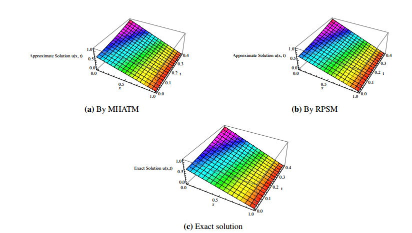
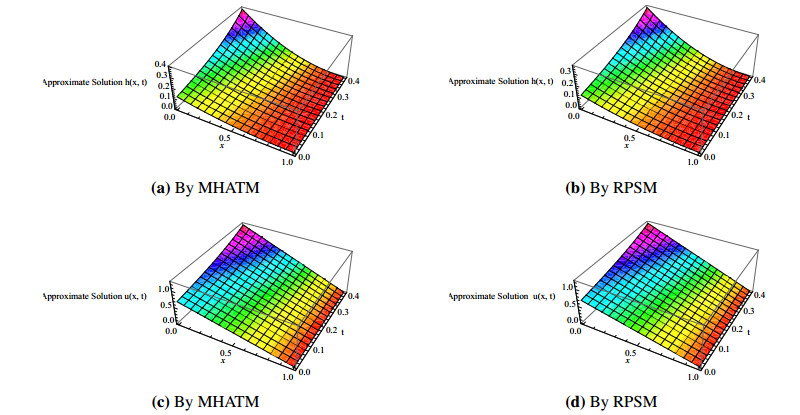
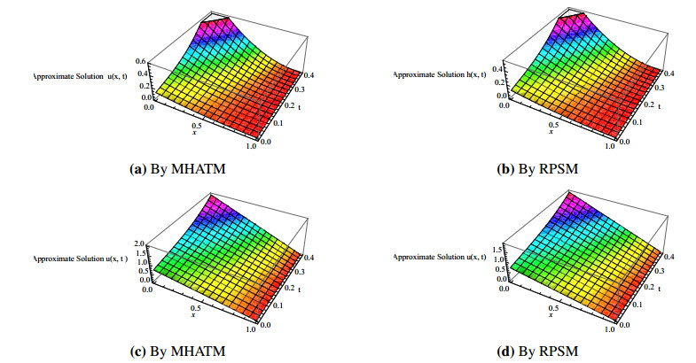
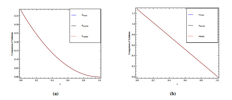
![]() |
1. | Fitriana Yuli Saptaningtyas, Wim T Van Horssen, Fajar Adi-Kusumo, Lina Aryati, On accurate asymptotic approximations of roots for polynomial equations containing a small, but fixed parameter, 2024, 9, 2473-6988, 28542, 10.3934/math.20241385 | |
2. | Chih-Wen Chang, Sania Qureshi, Ioannis K. Argyros, Francisco I. Chicharro, Amanullah Soomro, A modified two-step optimal iterative method for solving nonlinear models in one and higher dimensions, 2025, 229, 03784754, 448, 10.1016/j.matcom.2024.09.021 | |
3. | Mudassir Shams, Bruno Carpentieri, Chaos in Inverse Parallel Schemes for Solving Nonlinear Engineering Models, 2024, 13, 2227-7390, 67, 10.3390/math13010067 | |
4. | Mudassir Shams, Bruno Carpentieri, Efficient families of higher-order Caputo-type numerical schemes for solving fractional order differential equations, 2025, 124, 11100168, 337, 10.1016/j.aej.2025.02.111 | |
5. | Sania Qureshi, Ioannis K. Argyros, Higinio Ramos, Amanullah Soomro, Paras Nizamani, G Thangkhenpau, Sunil Panday, A stable optimal solver for nonlinear equations with semilocal convergence using majorizing sequences in banach spaces, 2025, 2254-3902, 10.1007/s40324-025-00402-x |
Method | MS | MM | ZPH | |||
Elapsed time | Iterations | Elapsed time | Iterations | Elapsed time | Iterations | |
ϑ1(ϰ) | 1.583536 | 25 | 0.456321 | 4 | 1.432156 | 7 |
ϑ2(ϰ) | 2.732514 | 23 | 0.632145 | 5 | 2.132564 | 7 |
Methods | ASm | Mm | Dm |
ZPH | 8.0m2+B | 6.0m2+B | 2.0m2+B |
MM | 6.0m2+B | 3.0m2+B | 2.0m2+B |
Method | CPU | ¯ς(5)1 | ¯ς(5)2 | ¯ς(5)3 | ¯ς(5)4 |
ZPH | 0.241 | 1.29e-17 | 1.62e-17 | 6.15e-32 | 4.16e-15 |
MM | 0.016 | 3.41e-51 | 1.15e-51 | 5.92e-53 | 5.82e-53 |
Method | CPU | ¯ς(17)1 | ¯ς(17)2 | ¯ς(17)3 | ¯ς(17)4 |
ZPHϑ1 | 2.1456 | 3.34e-07 | 2.43e-05 | 4.30e-07 | 8.35e-04 |
ZPHϑ2 | 3.1255 | 1.21e-03 | 0.32e-03 | 0.30e-08 | 1.13e-05 |
ZPHϑ3 | 2.9914 | 4.34e-05 | 2.31e-04 | 0.13e-03 | 4.35e-04 |
MMϑ1 | 1.1201 | 9.41e-34 | 4.3e-29 | 4.13e-32 | 7.81e-35 |
MMϑ2 | 1.32451 | 3.10e-32 | 2.3e-26 | 1.13e-18 | 8.03e-21 |
MMϑ3 | 0.93114 | 1.01e-33 | 2.3e-21 | 1.31e-19 | 8.73e-30 |
Method | CPU | ¯ς(17)1 | ¯ς(17)2 | ¯ς(17)3 |
ZPH | 0.1325 | 0.0200 | 0.0200 | 0.0030 |
MM | 0.0154 | 0.14e-09 | 9.15e-09 | 4.41e-09 |
Method | CPU | ¯ς(37)1 | ¯ς(37)2 | ¯ς(37)3 |
ZPHϑ1 | 5.4371 | 1.074e-20 | 3.398e-10 | 7.213e-18 |
ZPHϑ2 | 5.1351 | 2.087e-29 | 6.385e-11 | 0.321e-19 |
ZPHϑ3 | 3.1351 | 5.450e-27 | 7.378e-13 | 0.345e-17 |
MMϑ1 | 2.1221 | 0.494e-37 | 8.375e-30 | 3.345e-35 |
MMϑ2 | 1.8321 | 4.074e-35 | 0.378e-26 | 6.345e-35 |
MMϑ3 | 2.9321 | 6.0548e-31 | 1.378e-26 | 1378e-28 |
Method | CPU | ¯ς(6)1 | ¯ς(6)2 | ¯ς(6)3 | ¯ς(6)4 |
ZPH | 0.331 | 2.3e-23 | 2.3e-24 | 7.4e-33 | 3.1e-29 |
MM | 0.111 | 2.6e-30 | 2.6e-35 | 2.1e-35 | 2.3e-36 |
Method | CPU | ¯ς(11)1 | ¯ς(11)2 | ¯ς(11)3 | ¯ς(11)4 |
ZPHϑ1 | 2.1231 | 0.07e-30 | 2.23e-16 | 0.31e-18 | 8.73e-31 |
ZPHϑ2 | 2.4131 | 2.02e-30 | 1.32e-16 | 0.53e-18 | 1.53e-31 |
ZPHϑ3 | 3.1131 | 1.02e-30 | 5.35e-16 | 1.39e-18 | 8.03e-31 |
MMϑ1 | 1.0212 | 9.24e-41 | 4.53e-30 | 4.32e-32 | 7.18e-35 |
MMϑ2 | 1.8312 | 8.02e-47 | 2.30e-36 | 2.23e-28 | 8.23e-41 |
MMϑ3 | 1.7315 | 7.07e-48 | 2.37e-36 | 2.13e-28 | 1.32e-35 |
Method | CPU | ¯ς(7)1 | ¯ς(7)2 | ¯ς(7)3 | ¯ς(7)4 |
ZPH | 0.13121 | 3.02e-30 | 2.32e-16 | 2.32e-18 | 0.32e-31 |
MM | 0.02154 | 9.42e-36 | 4.13e-30 | 4.32e-32 | 7.81e-35 |
Method | CPU | ¯ς(10)1 | ¯ς(10)2 | ¯ς(10)3 | ¯ς(10)4 |
ZPHϑ1 | 2.031 | 3.50e-38 | 2.3e-18 | 4.38e-18 | 4.34e-33 |
ZPHϑ2 | 3.534 | 0.01e-39 | 2.3e-26 | 5.87e-18 | 3.53e-36 |
ZPHϑ3 | 4.1381 | 4.05e-35 | 4.31e-26 | 2.53e-17 | 2.34e-35 |
MMϑ1 | 3.0914 | 9.46e-46 | 0.30e-30 | 4.3e-32 | 7.85e-37 |
MMϑ2 | 1.0315 | 4.04e-45 | 2.35e-26 | 3.38e-28 | 8.13e-35 |
MMϑ3 | 2.1931 | 1.40e-41 | 4.35e-26 | 9.32e-29 | 1.32e-35 |
Method | CPU | ¯ς(6)1 | ¯ς(6)2 | ¯ς(6)3 | ¯ς(6)4 | ¯ς(6)5 | ¯ς(6)6 | ¯ς(6)7 | ¯ς(6)8 | ¯ς(6)9 |
ZPH | 0.431 | 3.0e-30 | 2.3e-25 | 0.0 | 0.0 | 0.0 | 2.3e-29 | 2.3e-35 | 0.0 | 0.0 |
MM | 0.221 | 9.4e-36 | 0.0 | 0.0 | 0.0 | 0.0 | 0.0 | 0.0 | 0.0 | 0.0 |
Method | CPU | ¯ς(10)1 | ¯ς(10)2 | ¯ς(10)3 | ¯ς(10)4 | ¯ς(10)5 | ¯ς(10)6 | ¯ς(10)7 | ¯ς(10)8 | ¯ς(10)9 |
ZPHϑ1 | 2.031 | 4.34e-23 | 3.50e-28 | 2.36e-18 | 4.38e-18 | 0.34e-23 | 0.51e-38 | 0.53e-28 | 1.31e-18 | 4.34e-33 |
ZPHϑ2 | 3.534 | 0.11e-29 | 2.31e-26 | 2.31e-26 | 5.87e-15 | 3.13e-26 | 0.01e-39 | 0.31e-36 | 1.87e-18 | |
ZPHϑ3 | 4.1381 | 2.34e-35 | 4.15e-25 | 4.61e-26 | 2.53e-17 | 4.05e-35 | 1.34e-35 | 4.05e-35 | 0.311e-36 | 1.34e-25 |
MMϑ1 | 3.0914 | 0.0 | 0.30e-30 | 1.30e-30 | 0.0 | 9.46e-46 | 0.0 | 0.0 | 5.3e-32 | 0.85e-47 |
MMϑ2 | 1.0315 | 0.0 | 2.35e-46 | 3.38e-48 | 8.13e-45 | 4.04e-45 | 0.0 | 0.0 | 0.0 | 8.13e-35 |
MMϑ3 | 2.1931 | 1.40e-47 | 4.35e-46 | 0.0 | 0.0 | 1.40e-41 | 4.35e-26 | 9.32e-29 | 1.32e-35 | 1.32e-35 |
Inital Vector | (0)ϰ1 | (0)ϰ2 | (0)ϰ3 | (0)ϰ4 | (0)ϰ5 | (0)ϰ6 | (0)ϰ7 | (0)ϰ8 | (0)ϰ9 |
ϑ(0)1 | 0.1234 | 0.2541 | 0.0415 | 0.04125 | 0.25410 | 025412 | 0.5412 | 0.0354 | 0..35214 |
ϑ(0)2 | 0.2134 | 0.5412 | 0.03251 | 0.05412 | 0.10351 | 0.0541 | 0.09854 | 0.0214 | 0.874515 |
ϑ(0)3 | 0.3251 | 0.6541 | 0.210 | 0.14521 | 0.2321 | 0.0012 | 0.5214 | 0.2145 | 0.022145 |