Gaseous and particulate emissions from the combustion of coal have been associated with adverse effects on human and environmental health, and have for that reason been subject to regulation by federal and state governments. Recent regulations by the United States Environmental Protection Agency have further restricted the emissions of acid gases from electricity generating facilities and other industrial facilities, and upcoming deadlines are forcing industry to consider both pre- and post-combustion controls to maintain compliance. As a result of these recent regulations, dry sorbent injection of trona to remove acid gas emissions (e.g. HCl, SO2, and NOx) from coal combustion, specifically 90% removal of HCl, was the focus of the current investigation. Along with the measurement of HCl, SO2, and NOx, measurements of particulate matter (PM), elemental (EC), and organic carbon (OC) were also accomplished on a pilot-scale coal-fired combustion facility.
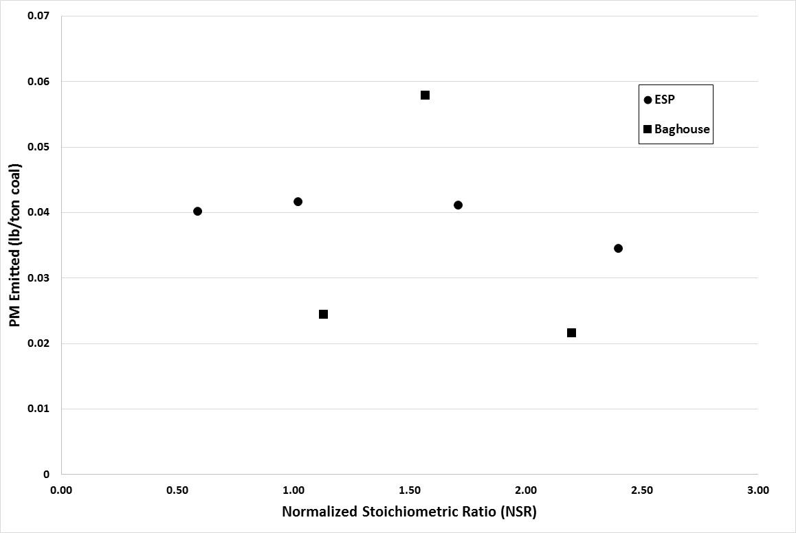
Gaseous and particulate emissions from a coal-fired combustor burning bituminous coal and using dry sorbent injection were the focus of the current study. From this investigation it was shown that high levels of trona were needed to achieve the goal of 90% HCl removal, but with this increased level of trona injection the ESP and BH were still able to achieve greater than 95% fine PM control. In addition to emissions reported, measurement of acid gases by standard EPA methods were compared to those of an infrared multi-component gas analyzer. This comparison revealed good correlation for emissions of HCl and SO2, but poor correlation in the measurement of NOx emissions.
1.
Introduction
Dengue is a viral disease transmitted mainly by Aedes mosquitoes, including Aedes aegypti and Aedes albopictus. Infected human beings carrying dengue viruses may get high fever, headaches, and skin rash, which may progress to dengue shock syndrome or dengue hemorrhagic fever. The annually reported dengue cases increased sharply from 2.2 million in 2010 to 3.2 million in 2015 [1]. More than 500, 000 people with severe dengue are hospitalized annually, and the case fatality percentage is about 2.5%. Due to the lack of commercially available vaccines for dengue control, traditional methods have been focused on vector control by heavy applications of insecticides and environmental management [2]. However, these programs have not prevented the spread of these diseases due to the rapid development of insecticide resistance [3] and the continual creation of ubiquitous breeding sites.
An innovational mosquito control method utilizes Wolbachia, an intracellular bacterium present in about 60% of insect species [4], including some mosquitoes. Wolbachia can induce cytoplasmic incompatibility (CI) in mosquitoes, which results in early embryonic death from matings between Wolbachia-infected males and females that are either uninfected or harbor a different Wolbachia strain [5,6]. In the world's largest "mosquito factory" located in Guangzhou, China, 20 million Wolbachia-infected males are produced each week. These mosquitoes have been released in several urban and suburb areas since 2015, and killed more than 95% mosquitoes on the Shazai island [7]. Motivated by the success and the challenge in field trials, the study on the complex Wolbachia spread dynamics has become a hot research topic. Various mathematical models have been developed, including models of ordinary differential equations [8,9,10], delay differential equations [9,11,12,13], impulsive differential equations [14], stochastic equations [15], and reaction-diffusion equations [16]. These models are mainly devoted to analyzing the threshold dynamics for population replacement with Wolbachia-infected female mosquitoes or CI-driven population suppression, which only included mosquito population into the models. However, it is usually a formidable task for complete population replacement or eradication in large-scale field trials, and we can only concede mosquito replacement/eradication to virus eradication by restricting the mosquito densities below the epidemic risk threshold.
To assess the efficacy of blocking dengue virus transmission by Wolbachia, a deterministic mathematical model of human and mosquito populations interfered by the circulation of a single dengue serotype was developed in the framework of SIER model [17]. This important study has inspired further development of compartmental models to analyze the transmission dynamics of dengue [18,19,20,21,22]. In this paper, we extend their efforts by incorporating the Wolbachia-infected male mosquito release into a compartmental model, where the infected males are maintained at a fixed ratio to the adult female mosquito population. We divide the mosquito population into three compartments: susceptible, exposed and infectious, and divide the human population into four compartments: susceptible, exposed, infectious and recovered. In particular, we include the respective extrinsic and intrinsic incubation periods (EIP and IIP) in the mosquito and human populations in our model. These periods have been shown to be crucial in clinical diagnosis, outbreak investigation, and dengue control [23], but have received relatively little attention [9,18]. Further, the release of Wolbachia-infected male mosquitoes is not effective immediately in sterilizing wild females due to the maturation delay between mating and emergence of adults [24]. To characterize the effect of EIP, IIP and the maturation delay on dengue transmission, we introduce three delays into our model.
The model treats IIP in humans, EIP in mosquitoes, and the maturation delay as three delays. We aim to find the threshold values of the release ratio for mosquito or virus eradication under the proportional release policy. By analyzing the existence and stability of disease-free equilibria, we obtain the sufficient and necessary condition on the existence of the disease-endemic equilibrium. Two threshold values of the release ratio $ \theta $, denoted by $ \theta_1^* $ and $ \theta_2^* $ with $ \theta_1^* > \theta_2^* $ are explicitly expressed. When $ \theta > \theta_1^* $, the mosquito population will be eradicated eventually. If it fails for mosquito eradication but $ \theta_2^* < \theta < \theta_1^* $, virus eradication is ensured together with the persistence of susceptible mosquitoes. When $ \theta < \theta_2^* $, the disease-endemic equilibrium emerges that allows dengue virus to circulate between humans and mosquitoes through mosquito bites. Sensitivity analysis of the threshold values in terms of the model parameters, and numerical simulations on several possible control strategies with different release ratios confirm the public awareness that reducing mosquito bites and killing adult mosquitoes are the most effective strategy to control the epidemic. Our model will provide new insights on the effectiveness of Wolbachia in reducing dengue at a population level.
2.
Model formulation
We divide adult mosquitoes into subetaoups of susceptible ($ S_M $), exposed ($ E_M $) and infectious ($ I_M $). Let $ N_M = S_M+E_M+I_M $ be the total number of mosquitoes. The human population is divided into four subpopulations: susceptible ($ S_H $), exposed (infected but not infectious, $ E_H $), infectious ($ I_H $), and recovered ($ R_H $). The total number of humans is denoted by $ N_H = S_H+E_H+I_H+R_H $. Without the bothering of the dengue virus, i.e., $ E_M = I_M = E_H = I_H = R_H = 0 $, we assume that mosquito and human populations follow the logistic growth [25] satisfying
where $ r_H $ and $ \mu_H $ are respectively the birth rate and the death rate of humans, and $ \kappa_H $ is a constant which leads the human carrying capacity to $ [(r_H-\mu_H)/r_H]\kappa_H $. Similarly, we set $ r_M $, $ \mu_M $, and $ \kappa_M $ as the birth rate, the death rate, and the carrying capacity parameter for mosquitoes. The prevalence of dengue virus disrupts the dynamics of humans and mosquitoes, which are split into $ S_H $, $ E_H $, $ I_H $, $ R_H $ and $ S_M $, $ E_M $, $ I_M $, respectively.
Dengue viruses can be transmitted from infectious mosquitoes to susceptible humans through bites. Let $ b $ be the average daily biting rate per female mosquito, and $ \beta_{MH} $ be the fraction of transmission from mosquitoes to humans. Then, susceptible humans acquire the infection at the rate $ [b\beta_{MH}I_M(S_H/N_H)] $, and we have
Let $ \tau_H $ be the intrinsic incubation period (IIP) in humans between infection and the onset of infectiousness. IIP is an important determinant of dengue transmission dynamics, which varies from 3 to 14 days. Exposed humans become infectious at the rate
With further assumption that infected but not infectious humans have the same death rate as that of susceptible humans, $ E_H $ follows
Let $ \gamma $ be the recovery rate of humans. Then for $ I_H $ and $ R_H $, we arrive at
where we disregard the negligible dengue mortality in humans [26] and set an identical mortality rate for humans.
With the release of Wolbachia-infected male mosquitoes, denoted by $ R(t) $ at time $ t $, the birth rate of mosquitoes is reduced from $ r_M $ to
Under random mating and equal sex determination, the probability of CI occurrence at time $ t $ is the proportion of Wolbachia-infected male mosquitoes among all male mosquitoes, i.e., $ R(t)/(R(t)+N_M(t)) $. However, there is a delay between the release of Wolbachia-infected males and the reduction of the wild mosquitoes which is caused by the maturation delay between mating and emergence of adult mosquitoes [24], denoted by $ \tau_e $. Hence, the number of susceptible mosquitoes that survive the maturation period is
The susceptible mosquitoes become exposed at a rate of $ [b\beta_{HM}S_M(I_H/N_H)] $, where $ \beta_{HM} $ is the fraction of virus transmission from infectious humans to susceptible mosquitoes through blood meals. Taking these considerations into account, we have
Exposed mosquitoes spend the extrinsic incubation period (EIP), denoted by $ \tau_M $, which is the viral incubation period between the time when a female mosquito takes a viraemia blood meal from an infectious human and the time when that mosquito becomes infectious [27], typically 8~12 days. EIP has been frequently recognized as a crucial component of dengue virus transmission dynamics [23]. In view of this point, the rate that exposed mosquitoes become infectious per unit time is $ [e^{-\mu_M\tau_M}b\beta_{HM}S_M(t-\tau_M) (I_H(t-\tau_M)/N_H(t-\tau_M))] $. Then the whole set of equations in our model ends with
for exposed and infectious mosquitoes, respectively.
Our purpose is to find the threshold values in terms of the release ratio for mosquito or virus eradication under the proportional release policy, where the Wolbachia-infected male mosquitoes is maintained in a fixed proportion to the adult female mosquito population, i.e.,
The explicit expressions of the threshold values are obtained as follows:
with $ \theta_1^* > \theta_2^* $. We get the following theorem.
Theorem 1. If $ \theta > \theta_1^* $, then eradication of mosquitoes occurs. If $ \theta_2^* < \theta < \theta_1^* $, then eradication of virus occurs. If $ \theta < \theta_2^* $, then there exists a unique disease-endemic equilibrium of system (2.1)-(2.7).
The proof of Theorem 1 is embodied in the analysis of the existence and stability of equilibrium points of system (2.1)-(2.7) in the following two sections, and we omit it here.
3.
Existence of equilibria
To determine the steady-state solutions of system (2.1)-(2.7), we set the right sides of (2.1)-(2.7) to zero and ignore the time lags to arrive at
Adding (3.1a) to (3.1d) together, we have
which yields
provided that $ \mu_H < r_H $ holds. Similarly, adding (3.1e) to (3.1g) together, we have
which leads to
Define the net reproductive numbers for humans and mosquitoes respectively by
Theorem 2. Assume that
Besides the zero equilibrium, system (2.1)-(2.7) admits two disease-free equilibrium points
Remark 1. The equilibrium point $ E_{01}^* $ corresponds to mosquito eradication as well as the infectious-free state for humans. The equilibrium point $ E_{02}^* $ biologically corresponds to the coexistence of mosquitoes and humans, without the infection of dengue virus, which more closely fits the actual situation. In the following discussion, we always assume that $ R_0^H > 1 $.
To find the disease-endemic equilibrium point of system (2.1)-(2.7), denoted by
we need to solve the algebraic equations (3.1a)-(3.1g). If we define the basic reproduction number by
then we obtain the existence of the disease-endemic equilibrium as follows.
Theorem 3. The unique disease-endemic equilibrium of system (2.1)-(2.7) exists if and only if $ R_0 > 1 $ and $ R_0^M > 1 $.
Proof. From (3.1d), we have
From (3.1b) and (3.1c), we respectively have
Hence we get the relation between $ E_H^* $ and $ I_H^* $ as
i.e.,
Recall that at any steady state, we have
Combining (3.1a) and (3.1c), one has
and hence
From (3.1f) by (3.1g), we have
Hence, we get the relation between $ E_M^* $ and $ I_M^* $ which reads as
Again, notice that at any steady state, we have
Then from (3.1e) and (3.1g), we arrive at
which leads to
From (3.5) to (3.9), to get the explicit expression of the disease-endemic equilibrium point, we only need to solve for $ I_H^* $ and $ I_M^* $. To this end, combining (3.1c) and (3.7), we have
Similarly, from (3.1g) and (3.9), we have
Tedious but direct computations from (3.10)-(3.11) offers a linear relation between $ I_M^* $ and $ I_H^* $ as
Plugging (3.12) into (3.10) and (3.11) yields the unique $ I_H^* $ and $ I_M^* $ as
It is easy to see from (3.5), (3.6), and (3.8) that $ R_H^* $, $ E_H^* $, and $ E_M^* $ are positive provided that $ I^*_M $ and $ I_H^* $ are positive. From (3.7) and (3.13), we have
always holds provided $ N^*_M > 0 $ and $ N_H^* > 0 $. Similarly, to guarantee $ S_M^* > 0 $, (3.9) requires again $ N^*_M > 0 $. From (3.9) and (3.14), with $ N^*_H > 0 $, we have
Hence, the disease-endemic equilibrium point exists if and only if
i.e., $ R_0 > 1 $. With the conclusion of Theorem 2, we complete the proof.
4.
Stability of equilibria
Because we are dealing with a system of delay differential equations, the characteristic equation has an infinite number of roots satisfying
where $ I $ is the identity matrix and the matrices $ J $, $ J_{\tau_H} $, $ J_{\tau_M} $ and $ J_{\tau_e} $ have entries that are the partial derivatives of the right sides of (2.1)-(2.7) with respect to, respectively,
Theorem 4. The disease-free equilibria $ E_{01}^* $ is locally asymptotically stable if and only if $ R_0^M < 1 $.
Proof. The matrices in (4.1) at $ E_{01}^* $ are
The characteristic matrix at $ E_{01}^* $ is $ \left(A∗01(λ)B∗010C∗01(λ)
\right) $ with
We firstly notice that when $ R_0^H > 1 $, $ \mu_H-r_H < 0 $. To prove the conclusion, we only need to prove that all roots of
have negative real parts if and only if $ R_0^M < 1 $. Recall Theorem 4.7 in Smith [28] which states that $ \lambda = a+be^{- \lambda \tau} $ has no roots with non-negative real parts if $ a+b < 0 $ and $ b\ge a $, irrelevant of the value of $ \tau > 0 $. By this theorem, we see that when
i.e., $ R_0^M < 1 $, all roots of (4.6) have negative real parts.
Next we prove that the condition (4.7) is also sufficient to exclude the possibility for (4.6) to have roots with non-negative real parts. To proceed, assume that $ \lambda = z_1+iz_2 $ with $ z_1\ge 0 $ is a solution of (4.6). Then
It is easy to see that if $ (z_1, z_2) $ satisfies (4.8)-(4.9), so does $ (z_1, -z_2) $. Without loss of generality, we assume that $ z_2\ge 0 $. Taking square of (4.8) and (4.9) and adding them together, we have
If $ z_2 = 0 $, then $ z_1 > 0 $ due to (4.7), and from (4.10), we have
a contradiction to (4.7). If $ z_2 > 0 $, from (4.10), we have
also a contradiction to (4.7). This completes the proof.
Remark 2. Theorem 4 implies that if the proportion of Wolbachia-infected males to wild mosquito population, $ \theta $, satisfies $ \theta > \theta_1^* $, then wild mosquitoes will be eradicated eventually, which has proved the first conclusion of Theorem 1.
Next we consider the stability of $ E_{02}^* $. The Jacobian matrices in (4.1) at $ E_{02}^* $ are
The characteristic matrix at $ E_{02}^* $ is $ \left(A∗02(λ)B∗02C∗02D∗02(λ)
\right) $ with
where
By direct computation, roots of (4.1) at $ E_{02}^* $ are $ \mu_H-r_H, \ -\mu_H $ together with roots of
where
On the roots of $ S_1(\lambda) = 0 $ and $ S_2(\lambda) = 0 $, we have the following two lemmas.
Lemma 4.1. All roots of $ S_1(\lambda) = 0 $ have negative real parts if and only if $ R_0^M > 1 $.
Proof. Notice that $ S_1(\lambda)\to -\infty $ as $ \lambda\to +\infty $. Then it is necessary to have $ S_1(0) < 0 $ to guarantee that all roots of $ S_1(\lambda) = 0 $ have negative real parts. Since
$ S_1(0) < 0 $ if $ R_0^M > 1 $. We claim that the condition $ R_0^M > 1 $ is also sufficient. In fact, assume that $ \lambda = \alpha+ i\beta $ satisfies $ S_1(\lambda) = 0 $. Then
Separating the real and imaginary parts yields
If $ (\alpha, \beta) $ satisfies (4.19)-(4.20), so does $ (z_1, -z_2) $. Without loss of generality, we assume that $ \beta\ge 0 $. If $ \alpha\ge 0 $, then $ e^{- \alpha \tau_e}\leq 1 $. Equation (4.19) implies that
and hence
a contradiction, which completes the proof.
Lemma 4.2. All roots of $ S_2(\lambda) = 0 $ have negative real parts if and only if $ R_0 < 1 $.
Proof. Notice that $ S_2(\lambda) $ is increasing with $ \lambda $, and $ S_2(\lambda)\to +\infty $ as $ \lambda\to +\infty $. Hence to make sure that all roots of $ S_2(\lambda) = 0 $ have negative real parts, the necessary condition is that $ S_2(0) > 0 $, that is,
i.e., $ R_0 < 1 $. We claim that condition (4.21) is also sufficient to guarantee that all roots of $ S_2(\lambda) = 0 $ have negative real parts. For notation simplicity, we define
Assume that $ \lambda = z_1+iz_2 $ is a solution of $ S_2(\lambda) = 0 $. Then
It is easy to see that if $ (z_1, z_2) $ is a solution of (4.22a)-(4.22b), so does $ (z_1, -z_2) $. Thus we can assume $ z_2 > 0 $. Next we prove that $ z_1 < 0 $ holds. If not, assume $ z_1 = 0 $. Then (4.22a)-(4.22b) are reduced to
which produces
Therefore,
a contradiction to (4.21). On the other hand, if $ z_1 > 0 $, then from (4.22a)-(4.22b), we have
Therefore,
also a contradiction to (4.21). This completes the proof.
From Lemmas 4.1 and 4.2, we have
Theorem 5. The disease-free equilibrium point $ E_{02}^* $, if exists, is locally asymptotically stable.
Results on the existence and stability of equilibria for system (2.1)-(2.2) are summarized in Table 1. Noticing the fact that
we conclude that Theorem 1 holds.
5.
Numerical implications on mosquito/dengue control
5.1. Sensitivity analysis of $ R_0 $
The basic reproduction number $ R_0 $ is a function of the parameters listed in Table 2.
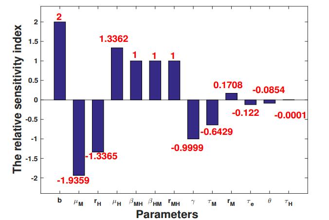
To estimate the response of $ R_0 $ to different parameters, following the procedure in [20], we define the relative sensitivity index of $ R_0 $ with respect to each parameter $ p $ in Table 2 by
where $ p^* $ is taken as the baseline value in Table 2 which also yields $ R_0^* = 1.5869 $. The relative sensitivity indices are shown in Figure 1 which are ranked in their absolute values. It turns out that avoiding mosquito bites through physical and chemical means or a combination of both is the most direct and effective method to reduce the transmission of dengue virus, which has comparable performance of elevating the death rate of mosquitoes, $ \mu_M $. Compared with the parameter $ \mu_M $, the birth rate of mosquitoes, $ r_M $, has much less contribution to $ R_0 $. The elevation of $ R_0 $ due to the increase of $ \mu_H $ can be almost equally offset by the decrease of $ r_H $. Parameters $ \beta_{MH} $, $ \beta_{HM} $, the ratio of the carrying capacities of mosquitoes to humans, $ r_{MH} $, and the recovery rate of humans $ \gamma $, contribute equally to $ R_0 $. Among the three delay parameters, the extrinsic incubation period of mosquitoes, $ \tau_M $, is the most sensitive parameter, while the intrinsic incubation period of humans, $ \tau_H $, is the least sensitive one. Unexpectedly, the release ratio, $ \theta $, only plays a minor role in controlling the basic reproduction number. The most likely reason is that the baseline value of $ \theta $ is set as 1, much smaller than the release ratio in field trials. Coincidentally, further computation shows that when the release ratio is increased from 5 to 6, the basic reproduction number is decreased from 1.0447 to 0.9092$ (<1) $. This observation is in line with our claim that for mosquito eradication or virus eradication, the optimal release ratio of Wolbachia-infected male mosquitoes to wild males is about 5 to 1 [9,33].
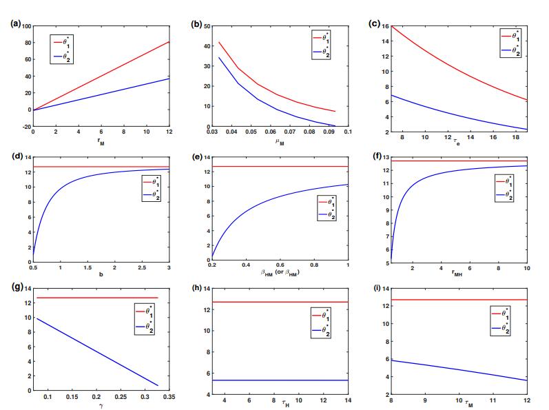
5.2. Dynamics of $ \theta_1^* $ and $ \theta_2^* $
Theorem 2.1 shows that $ \theta_1^* $ is the threshold value for mosquito eradication. If mosquito eradication fails, then $ \theta_2^* $ is the threshold value for virus eradication. Dynamics of $ \theta_1^* $ and $ \theta_2^* $ are shown in Figure 2, which are in terms of the designated parameter while letting other parameters in system (2.1)-(2.7) be fixed as the baseline values in Table 2. The threshold values $ \theta_1^* $ and $ \theta_2^* $ increase as $ r_M $ increase; see Figure 2(a), which decrease as $ \mu_M $ or $ \tau_e $ decrease; see Figure 2(b) and (c). The threshold value $ \theta_1^* $ is fixed at 12.7072 when $ r_M $, $ \mu_M $ and $ \tau_e $ are fixed. In terms of $ b $, $ \beta_{HM} $, $ \beta_{MH} $, and $ r_{MH} $, the threshold $ \theta_2^* $ presents a quasi-logistic growth mode; see Figure 2(d), (e), and (f). The threshold $ \theta_2^* $ is a linear decreasing function of $ \gamma $ or $ \tau_M $; see Figure 2(g) and (i). When $ \tau_H $ lies between 3 and 14, it only brings a negligible change of $ \theta_2^* $; see Figure 2(h) which is consistent with the observation in Figure 1 that the relative sensitivity index of $ \tau_H $ is very close to 0.
5.3. Dynamics of mosquitoes and/or viruses under different release ratios
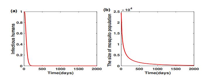
Given the baseline values in Table 2, we have
which offer the threshold values of mosquito and virus eradication, respectively. We initiate system (2.1)-(2.7) with one infectious human, and a mosquito population size about $ 25, 000 $ with one infectious mosquito. Figure 3 shows that if we take the release ratio $ \theta = 13 > \theta_1^* $, then both the virus and mosquito will eventually be eradicated. When the production of Wolbachia-infected male mosquitoes fails to meet $ \theta_1^* $, we can only concede mosquito eradication to virus eradication.
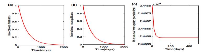
Figure 4 shows that the release ratio $ \theta = 6 $ successfully clears the virus, together with the persistence of mosquito populations. However, further lower of the release ratio to $ 2 $ which is less than the threshold value $ \theta_2^* $ can neither clear virus nor eradicate mosquitoes. To see this, we initiate system (2.1)-(2.7) near the disease-endemic equilibrium point $ E^* $, with
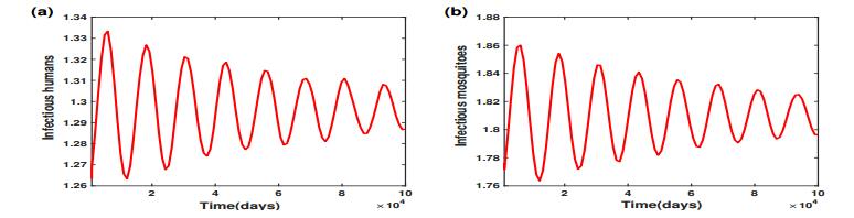
When $ \theta = 2 $, Figure 5 shows that the number of infectious humans oscillates in the vicinity of their steady-state $ I_H^*\approx 1.2958 $, and the number of infectious mosquitoes oscillates in the vicinity of their steady-state $ I_M^*\approx 1.8095 $.
6.
Conclusions
Dengue fever is one of the most common mosquito-borne viral diseases. Due to the lack of commercially available vaccines and efficient clinical cures, traditional methods have been focused on vector control by heavy applications of insecticides and environmental management. However, these programs have not prevented the spread of these diseases due to the rapid development of insecticide resistance and the continual creation of ubiquitous larval breeding sites. One novel dengue control method involves the intracellular bacterium Wolbachia, whose infection in Aedes aegypti or Aedes albopictus, the major mosquito vector of dengue virus, can greatly reduce the virus replication in mosquitoes. Wolbachia can also induce cytoplasmic incompatibility (CI) in mosquitoes, which results in early embryonic death from matings between Wolbachia-infected males and females that are either uninfected or harbor a different Wolbachia strain.
CI mechanism drives Wolbachia-infected male mosquitoes as a new weapon to suppress or eradicate wild females. However, complete population eradication in large-scale field trials is usually formidable, and we can only concede mosquito eradication to virus eradication by restricting the mosquito densities below the epidemic critical threshold. Motivated by the success and the challenge in field trials, we developed a deterministic mathematical model of human and mosquito populations interfered by the circulation of a single dengue serotype in the framework of SIER model to assess the efficacy of blocking dengue virus transmission by Wolbachia. We extended the SIER model by incorporating the Wolbachia-infected male mosquito release, where the infected males are maintained at a fixed ratio to the adult female mosquito population. Furthermore, the extrinsic incubation period in mosquito (EIP), the intrinsic incubation period in human (IIP), and the maturation delay between mating and emergence of adult mosquitoes were embedded as three delays in our model.
The threshold values of the release ratio $ \theta $ for mosquito or virus eradication were found by seeking the sufficient and necessary condition on the existence of the disease-endemic equilibrium. Two explicit expressions on threshold values of $ \theta $, denoted by $ \theta_1^* $ and $ \theta_2^* $ with $ \theta_1^* > \theta_2^* $, were obtained. When $ \theta > \theta_1^* $, the mosquito population will be eradicated eventually. If it fails for mosquito eradication but $ \theta_2^* < \theta < \theta_1^* $, virus eradication is ensured together with the persistence of susceptible mosquitoes. When $ \theta < \theta_2^* $, the emergence of the disease-endemic equilibrium makes dengue virus circulation between humans and mosquitoes possible. Sensitivity analysis of the threshold values showed that avoiding mosquito bites through physical and chemical means is the most direct and effective method to reduce the transmission of dengue virus, which has comparable performance of elevating the death rate of mosquitoes. Results from numerical simulations also confirmed our previous claim that for mosquito eradication or virus eradication, the optimal release ratio of Wolbachia-infected male mosquitoes to wild males is about 5 to 1.
Acknowledgements
This work was supported by National Natural Science Foundation of China (11826302, 11631005, 11871174), Program for Changjiang Scholars and Innovative Research Team in University (IRT_16R16) and Science and Technology Program of Guangzhou (201707010337).
Conflict of interest
The authors have declared that no competing interests exist.


 DownLoad: