Loading [MathJax]/jax/element/mml/optable/GeneralPunctuation.js
Review Special Issues

Alzheimer’s Disease: A short introduction to the calmodulin hypothesis

  • Received: 21 August 2019 Accepted: 28 September 2019 Published: 12 October 2019
  • At the cellular level, Alzheimer’s disease (AD) is characterized by the presence of intracellular plaques containing amyloid beta (Aβ) protein and neurofibrillary tangles consisting of phospho-tau (p-tau). These biomarkers are considered to contribute, at least in part, to the neurodegenerative events of the disease. But the accumulation of plaques and tangles is widely considered to be a later event with other factors likely being the cause of the disease. Calcium dysregulation—the unregulated accumulation of calcium ions—in neurons is an early event that underlies neurodegeneration. In 2002, O’Day and Myre extended this “Calcium Hypothesis” to include calmodulin (CaM) the primary target of calcium, suggesting the “Calmodulin Hypothesis” as an updated alternative. Here we overview the central role of CaM in the formation of the classic hallmarks of AD: plaques and tangles. Then some insight into CaM’s binding to various risk factor proteins is given followed by a short summary of specific receptors and channels linked to the disease that are CaM binding proteins. Overall, this review emphasizes the diversity of Alzheimer’s-linked CaM-binding proteins validating the hypothesis that CaM operates critically at all stages of the disease and stands out as a potential primary target for future research.

    Citation: Danton H. O’Day. Alzheimer’s Disease: A short introduction to the calmodulin hypothesis[J]. AIMS Neuroscience, 2019, 6(4): 231-239. doi: 10.3934/Neuroscience.2019.4.231

    Related Papers:

    [1] Minzhi Wei . Existence of traveling waves in a delayed convecting shallow water fluid model. Electronic Research Archive, 2023, 31(11): 6803-6819. doi: 10.3934/era.2023343
    [2] Hami Gündoğdu . RETRACTED ARTICLE: Impact of damping coefficients on nonlinear wave dynamics in shallow water with dual damping mechanisms. Electronic Research Archive, 2025, 33(4): 2567-2576. doi: 10.3934/era.2025114
    [3] Yuchen Zhu . Blow-up of solutions for a time fractional biharmonic equation with exponentional nonlinear memory. Electronic Research Archive, 2024, 32(11): 5988-6007. doi: 10.3934/era.2024278
    [4] Yong Zhou, Jia Wei He, Ahmed Alsaedi, Bashir Ahmad . The well-posedness for semilinear time fractional wave equations on $ \mathbb R^N $. Electronic Research Archive, 2022, 30(8): 2981-3003. doi: 10.3934/era.2022151
    [5] José Luiz Boldrini, Jonathan Bravo-Olivares, Eduardo Notte-Cuello, Marko A. Rojas-Medar . Asymptotic behavior of weak and strong solutions of the magnetohydrodynamic equations. Electronic Research Archive, 2021, 29(1): 1783-1801. doi: 10.3934/era.2020091
    [6] Fanqi Zeng, Cheng Jin, Peilong Dong, Xinying Jiang . Cheng-Yau type gradient estimates for $ \Delta_f v^{\tau}+\lambda(x)v^l = 0 $ on smooth metric measure spaces. Electronic Research Archive, 2025, 33(7): 4307-4326. doi: 10.3934/era.2025195
    [7] Meng Wang, Naiwei Liu . Qualitative analysis and traveling wave solutions of a predator-prey model with time delay and stage structure. Electronic Research Archive, 2024, 32(4): 2665-2698. doi: 10.3934/era.2024121
    [8] Chang Hou, Hu Chen . Stability and pointwise-in-time convergence analysis of a finite difference scheme for a 2D nonlinear multi-term subdiffusion equation. Electronic Research Archive, 2025, 33(3): 1476-1489. doi: 10.3934/era.2025069
    [9] Ya Tian, Jing Luo . Boundedness and large time behavior of a signal-dependent motility system with nonlinear indirect signal production. Electronic Research Archive, 2024, 32(11): 6301-6319. doi: 10.3934/era.2024293
    [10] Pan Zhang, Lan Huang . Stability for a 3D Ladyzhenskaya fluid model with unbounded variable delay. Electronic Research Archive, 2023, 31(12): 7602-7627. doi: 10.3934/era.2023384
  • At the cellular level, Alzheimer’s disease (AD) is characterized by the presence of intracellular plaques containing amyloid beta (Aβ) protein and neurofibrillary tangles consisting of phospho-tau (p-tau). These biomarkers are considered to contribute, at least in part, to the neurodegenerative events of the disease. But the accumulation of plaques and tangles is widely considered to be a later event with other factors likely being the cause of the disease. Calcium dysregulation—the unregulated accumulation of calcium ions—in neurons is an early event that underlies neurodegeneration. In 2002, O’Day and Myre extended this “Calcium Hypothesis” to include calmodulin (CaM) the primary target of calcium, suggesting the “Calmodulin Hypothesis” as an updated alternative. Here we overview the central role of CaM in the formation of the classic hallmarks of AD: plaques and tangles. Then some insight into CaM’s binding to various risk factor proteins is given followed by a short summary of specific receptors and channels linked to the disease that are CaM binding proteins. Overall, this review emphasizes the diversity of Alzheimer’s-linked CaM-binding proteins validating the hypothesis that CaM operates critically at all stages of the disease and stands out as a potential primary target for future research.


    Consider the equation

    $ ututxx+βux+muux=3αuxuxx+αuuxxx, $ (1.1)

    in which constants $ m > 0 $, $ \alpha > 0 $, and $ \beta\in\mathbb{R} $. Equation (1.1) characterizes the hydrodynamical dynamics of shallow water waves and is a special model derived in Constantin and Lannes [1]. In fact, the nonlinear shallow water wave model holds great significance for the scientific community due to its application in tsunami modeling and forecasting, a critical scientific problem with global implications for coastal communities. The investigation of shallow water wave equations may aid scientists in comprehending and predicting the behavior of tsunamis.

    If $ m = \frac{3}{2} $, $ \beta = -1 $, and $ \alpha = \frac{3}{2} $, Eq (1.1) reduces to the Fornberg$ - $Whitham (FW) model [2,3]

    $ ututxx+32uux=ux+92uxuxx+32uuxxx. $ (1.2)

    Many works have been carried out to discuss various dynamical behaviors of the FW equation. Sufficient and necessary conditions, guaranteeing that the wave breaking of Eq (1.2) happens, are found out in Haziot [4]. The sufficient conditions of wave breaking and discontinuous traveling wave solutions to the FW model are considered in H$ \ddot{o} $rmann[5,6]. The continuity solutions of Eq (1.2) in Besov space are explored in Holmes and Thompson [7]. The H$ \ddot{o}lder $ continuous solutions to the FW model are in detail investigated in Holmes [8]. Ma et al. [9] provide sufficient conditions to ensure the occurrence of wave breaking for a range of nonlocal Whitham type equations. On the basis of $ L^2(\mathbb{R}) $ conservation law, Wu and Zhang [10] investigate the wave breaking of the Fornberg$ - $Whitham equation. Comparing to the previous wave breaking results for the FW model, Wei [11] gives a novel sufficient condition to guarantee that the wave breaking for Eq (1.2) happens.

    Suppose that $ m = 4 $, $ \beta = 0 $, and $ \alpha = 1 $, Eq (1.1) becomes the well-known Degasperis$ - $Procesi (DP) equation [12]

    $ ututxx+4uux=3uxuxx+uuxxx. $ (1.3)

    Many works have been carried out to study the dynamical characteristics of Eq (1.3). For instances, the integrability of the DP equation is derived in Degasperis and Procesi [12] and Degasperis et al. [13]. Escher et al. [14] investigate the existence of global weak solutions for the DP model. Liu et al. [15] prove the well-posedness of global strong solutions and blow-up phenomena for Eq (1.3) under certain conditions. Yin [16] considers the Cauchy problem for a periodic generalized Degasperis$ - $Procesi model. The large-time asymptotic behavior of the periodic entropy solutions for the DP equation is discussed in Conclite and Karlsen [17]. Various kinds of traveling wave solutions for Eq (1.3) are presented in [18,19,20]. In the Sobolev space $ H^s(\mathbb{R}) $ with $ s > \frac{3}{2} $, Lai and Wu [21] discuss the local existence for a partial differential equation involving the DP and Camassa$ - $Holm(CH) models. The investigation of wave speed for the DP model is carried out in Henry [22]. The dynamical properties of CH equations are presented in [23,24,25,26]. For dynamical features of other nonlinear models, which are closely relevant to the DP and FW models, we refer the reader to [27,28,29,30].

    As we know, the $ L^2 $ conservation law derived from the DP or FW equation takes an essential role in investigating the dynamical features of the DP and FW models. We derive that Eq (1.1) possesses the following $ L^2 $ conservation law:

    $ R1+ξ2mα+ξ2|ˆu(ξ)|2dξ=R1+ξ2mα+ξ2|^u0(ξ)|2dξ∼∥u02L2(R), $ (1.4)

    where $ u(0, x) = u_0\in H^s(\mathbb{R}) $ endowed with the index $ s > \frac{3}{2} $ is the initial value of $ u $.

    A natural question is that as the shallow water wave model (1.1) generalizes the famous Fornberg$ - $Whitham equation (1.2) and Degasperis$ - $Procesi model (1.3), what kinds of dynamical characteristics of DP and FW models still hold for Eq (1.1). For this purpose, the key element of this work is that we derive $ L^2(\mathbb{R}) $ conservation law for (1.1). Using (1.4) and the technique of transport equation, we establish the boundedness of the solutions for Eq (1.1). Employing the approach called doubling the space variable in Kru$ \check{z} $kov [31], we investigate the $ L^1(\mathbb{R}) $ stability of short-time strong solutions provided that $ u_0(x) $ belongs to the space $ H^s(\mathbb{R})\cap L^1(\mathbb{R}) $ with $ s > \frac{3}{2} $. To our knowledge, this $ L^1(\mathbb{R}) $ stability of Eq (1.1) has never been established in literatures.

    The organization of this job is that Section 2 prepares several Lemmas. The $ L^1(\mathbb{R}) $ stability of short time solution to Eq (1.1) is established in Section 3.

    For the nonlinear shallow water wave equation (1.1), we write out its initial problem

    $ {ututxx+βux+muux=3αuxuxx+αuuxxx,u(0,x)=u0(x). $ (2.1)

    Utilizing inverse operator $ \mathbb{A}^{-2} = (1-\frac{\partial^2}{\partial x^2})^{-1} $, we obtain the equivalent form of (2.1), which reads as

    $ {ut+αuux=βA2ux+αm2A2(u2)x,u(0,x)=u0(x). $ (2.2)

    In fact, for any function $ D(x)\in L^{r}(\mathbb{R}) $ with $ 1\leq r\leq \infty $, we have

    $ A2D(x)=12Re|xz|D(z)dz. $

    Writing $ Q_u = \beta\mathbb{A}^{-2}u+\frac{m-\alpha}{2}\mathbb{A}^{-2}(u^2) $ and $ J_u = \beta\mathbb{A}^{-2}\partial_xu+\frac{m-\alpha}{2}\partial_x\mathbb{A}^{-2}(u^2) $ yields

    $ ut+α2(u2)x+Ju=0. $ (2.3)

    We define $ L^{\infty} = L^{\infty}(\mathbb{R}) $ with the standard norm $ \parallel h\parallel_{L^{\infty}} = \inf\limits_{m(e) = 0}\sup\limits_{x\in \mathbb{R}\backslash e}|h(t, x)| $. For any real number $ s $, we let $ H^s = H^s(\mathbb{R}) $ denote the Sobolev space with the norm defined by

    $ hHs=((1+|ξ|2)s|ˆh(t,ξ)|2dξ)12<, $

    where $ \hat{h}(t, \xi) = \int_{-\infty}^{\infty}e^{-ix\xi}h(t, x)dx $. For $ T > 0 $ and nonnegative number $ s $, let $ C([0, T);H^s(\mathbb{R}) $ denote the Frechet space of all continuous $ H^s $-valued functions on $ [0, T) $.

    Lemma 2.1. ([21]) Provided that $ s > \frac{3}{2} $ and initial value $ u_0(x)\in H^s(\mathbb{R}) $, then there has a unique solution $ u $ which belongs to the space $ C([0, T);H^s(\mathbb{R}))\cap C^1([0, T);H^{s-1}(\mathbb{R})) $, in which $ T $ represents maximal existence time for solution $ u $*.

    *In the sense of Lemma 2.1, for $ s > \frac{3}{2} $, the maximal existence time $ T $ means $ \lim\limits_{t\rightarrow T}\parallel u(t, \cdot) \parallel_{H^s(\mathbb{R})} = \infty $.

    Lemma 2.2. Suppose that $ m > 0 $, $ \alpha > 0 $, $ u_0\in H^s(\mathbb{R}) $, and $ s > \frac{3}{2} $. Let $ u $ be the solution of (2.1). Set $ y = u-\frac{\partial^2u}{\partial x^2} $ and $ Y = (\frac{m}{\alpha}-\frac{\partial^2}{\partial x^2})^{-1}u $. Then

    $ RyYdx=R1+ξ2mα+ξ2|ˆu(ξ)|2dξ=R1+ξ2mα+ξ2|^u0(ξ)|2dξ∼∥u02L2(R). $ (2.4)

    Moreover,

    $ {uL2αmu0L2,ifmα1,uL2mαu0L2,ifmα1. $ (2.5)

    Proof. We have $ u = \frac{m}{\alpha}Y-\partial_{xx}^2Y $ and $ \partial_{xx}^2Y = \frac{m}{\alpha}Y-u $. Utilizing integration by parts and Eq (1.1) yields

    $ ddtRyYdx=RytYdx+RyYtdx=2RYytdx=2R[(m2u2)xβux+α23xxx(u2)]Ydx=2R[(m2u2)xYβuxY+α2(u2)x2xxY]dx=R[(mu2)xY2βuxY+α(u2)x(mαYu)]dx=R(2βuxYα(u2)xu)dx=2βRuYxdx=2βR(mαY2xxY)Yxdx=0. $

    Utilizing the above identity and the Parserval identity gives rise to (2.4). Inequality (2.5) is derived directly from (2.4).

    For each time $ t\in[0, T) $, we write the transport system

    $ {qt=αu(t,q),q(0,x)=x. $ (2.6)

    The next lemma demonstrates that $ q(t, x) $ possesses the feature of increasing diffeomorphism.

    Lemma 2.3. Provided that $ T $ is defined as in Lemma 2.1 and $ u_0\in H^s(\mathbb{R}) $ endowed with $ s\geq 3 $, then system (2.6) possesses a unique $ q $ belonging to $ C^1([0, T)\times \mathbb{R}) $. In addition, $ q_x(t, x) > 0 $ in the region $ [0, T)\times \mathbb{R} $.

    Proof. Employing Lemma 2.1 derives that $ u_x\in C^2(\mathbb{R}) $ and $ u_t\in C^1[0, T) $ if $ (t, x)\in [0, T)\times \mathbb{R} $. Subsequently, it is concluded that solution $ u(t, x) $ and its slope $ u_x(t, x) $ possess boundness and are Lipschitz continuous in the region $ [0, T)\times \mathbb{R} $. Using the theorem of existence and uniqueness for ODE guarantees that system (2.6) possesses a unique solution $ q\in C^1([0, T)\times \mathbb{R}) $.

    Making use of system (2.6) gives rise to $ \frac{d}{dt}q_x = \alpha u_x(t, q)q_x $ and $ q_x(0, x) = 1 $. Thus, we have

    $ qx(t,x)=et0αux(τ,q(τ,x))dτ. $

    If $ T' < T $, we acquire

    $ \sup\limits_{(t,x)\in [0,T')\times R}|u_x(t, x)| < \infty, $

    implying that it must have a constant $ C_0 > 0 $ to ensure $ q_x(t, x)\geq e^{-C_0t} $. The proof is finished.

    For writing concisely in the following discussions, we utilize notations $ L^\infty = L^\infty(\mathbb{R}) $, $ L^1 = L^1(\mathbb{R}) $, and $ L^2 = L^2(\mathbb{R}) $.

    Lemma 2.4. Assume $ t\in [0, T] $, $ s > \frac{3}{2} $, and $ u_0\in H^s(\mathbb{R}) $. Then

    $ u(t,x)L≤∥u0L+(|β|c02u0L2+|αm|c204u02L2)t, $ (2.7)

    in which $ c_0 = \max\Big(\sqrt{\frac{\alpha}{m}}, \sqrt{\frac{m}{\alpha}}\Big) $.

    Proof. Set $ \eta(x) = \frac{1}{2}e^{-\mid x\mid} $. Utilizing the density arguments utilized in [15], we only need to deal with the case $ s = 3 $ to verify Lemma 2.4. For $ u_0\in H^3(\mathbb{R}) $, using Lemma 2.1 ensures the existence of $ u $ belonging to $ H^3(\mathbb{R}) $. Applying system (2.2) arises

    $ ut+αuux=(αm)η(uux)βηux, $ (2.8)

    where $ \star $ stands for the convolution. Using $ \int_{\mathbb{R}}e^{2|x-z|}dz = 1 $, we acquire

    $ |η(x)ux|=12|xex+zu(t,z)dz+xexzu(t,z)dz|12Re|xz||u(t,z)|dz12(Re2|xz|dz)12(Ru2(t,z)dz)1212uL2c02u0L2. $ (2.9)

    We have

    $ |η(uux)|=|12exzuuzdz|=12|xex+zuuzdz+12+xexzuuzdz|=|14xexzu2dz+14xexzu2dz|14exzu2dz14c20u02L2 $ (2.10)

    and

    $ du(t,q(t,x))dt=ut(t,q(t,x))+ux(t,q(t,x))dq(t,x)dt=ut(t,q(t,x))+αuux(t,q(t,x)). $ (2.11)

    Combining with (2.8)–(2.11) and Lemma 2.2 gives rise to

    $ du(t,q(t,x))dt∣≤|mα|4eq(t,x)zu2dz+βηux|mα|4u2dz+|β|2eq(t,x)zuzdz|mα|4u2L2+|β|2uL2|β|c02u0L2+|αm|c204u02L2. $ (2.12)

    From (2.12), we have

    $ {du(t,q(t,x))dt|β|c02u0L2+|αm|c204u02L2,du(t,q(t,x))dt(|β|c02u0L2+|αm|c204u02L2). $ (2.13)

    Integrating (2.13) on the interval $ [0, t] $ yields

    $ {u(t,q(t,x))u0(|β|c02u0L2+|αm|c204u02L2)t,u(t,q(t,x))u0(|β|c02u0L2+|αm|c204u02L2)t. $ (2.14)

    From the first inequality in (2.14), we have

    $ u(t,q(t,x))L(|β|c02u0L2+|αm|c204u02L2)t+u0L. $ (2.15)

    Using the second inequality in (2.14) gives rise to

    $ |u(t,q(t,x))||u0(|β|c02u0L2+|αm|c204u02L2)t.|(|β|c02u0L2+|αm|c204u02L2)t|u0|, $

    from which we have

    $ u(t,q(t,x))L(|β|c02u0L2+|αm|c204u02L2)tuL. $ (2.16)

    Utilizing (2.15) and (2.16), we obtain

    $ u(t,q(t,x))L≤∥u0L+(|β|c02u0L2+|αm|c204u02L2)t. $ (2.17)

    Utilizing Lemma 2.3 and (2.17) yields (2.7).

    Lemma 2.5. If $ u_0\in L^2(\mathbb{R}) $, then

    $ {Qu(t,)L(R)|β|c02u0L2+|αm|c204u02L2,Ju(t,)L(R)|β|c02u0L2+|αm|c204u02L2, $ (2.18)

    in which $ c_0 = \max\Big(\sqrt{\frac{\alpha}{m}}, \sqrt{\frac{m}{\alpha}}\Big) $.

    Proof. From (2.3), we have

    $ Qu=mα4Re|xz|u2(t,z)dz+β2Re|xz|u(t,z)dz, $ (2.19)
    $ Ju=mα4Re|xz|sgn(zx)u2(t,z)dz+β2Re|xz|sgn(zx)u(t,z)dz. $ (2.20)

    Utilizing (2.9), (2.19), (2.20), Lemma 2.2, and the Schwartz inequality, we obtain (2.18).

    Lemma 2.6. Let $ u_0, v_0\in H^s(\mathbb{R}), s > \frac{3}{2} $. Provided that functions $ u $ and $ v $ satisfy system (2.2), for any $ g(t, x)\in C_0^{\infty}([0, \infty)\times (-\infty, \infty)) $, then

    $ |Ju(t,x)Jv(t,x)||g(t,x)|dxc(1+t)|u(t,x)v(t,x)|dx, $ (2.21)

    in which $ c > 0 $ depends on $ m, \alpha, \beta, g, \parallel u_0 \parallel_{L^2} $ and $ \parallel v_0 \parallel_{L^2} $.

    Proof. Applying the Tonelli Theorem and Lemmas 2.2 and 2.4 gives rise to

    $ |Ju(t,x)Jv(t,x)||g(t,x)|dx|β|2e|xz||sgn(zx)||uv||g(t,x)|dzdx+|mα|2|xA2(u2u2)||g(t,x)|dxc|uv|dze|xz||g(t,x)|dx+|mα|4|e|xz||sgn(zx)||u2v2|dz|g(t,x)|dx|c|u(t,z)v(t,z)|dz+|mα|4|(uv)(u+v)|dz||g(t,x)|dx|c(1+t)|u(t,z)v(t,z)|dz, $

    from which we acquire (2.21).

    Suppose that function $ \gamma(y) $ is infinitely differentiable on $ \mathbb{R} $ such that $ \gamma(y)\geq 0 $, $ \gamma(y) = 0 $ when $ |y|\geq 1 $, and $ \int_{-\infty}^\infty \gamma(y)dy = 1 $. For arbitrary constant $ h > 0 $, set $ \gamma_h(y) = \frac{\gamma(h^{-1}y)}{h}\geq 0 $. Thus, $ \gamma_h(y) $ belongs to $ C^\infty(-\infty, \infty) $ and

    $ |γh(y)|ch,γh(y)dy=1;γh(y)=0if|y|h. $

    Suppose that $ G(x) $ is locally integrable in $ \mathbb{R} $. Its mean function is written as

    $ Gh(x)=1hγ(xyh)G(y)dy,h>0. $

    For the Lebesgue point $ x_0 $ of $ G(x) $, it has

    $ limh01h|xx0|h|G(x)G(x0)|dx=0. $ (2.22)

    If $ x $ is an arbitrary Lebesgue point of $ G(x) $, it has $ \lim\limits_{h\rightarrow 0}G^h(x) = G(x) $. Provided that point $ x $ is not Lebesque point of $ G(x) $, (2.22) always holds. Thus, $ G^h(x)\rightarrow G(x) $ ($ h\rightarrow 0 $) is valid almost everywhere.

    We illustrate the notation of a characteristic cone. Suppose that $ N > \max\limits_{t\in [0, T]}\parallel W(t, \cdot)\parallel_{L^\infty} < \infty $, $ 0\leq t\leq T_0 = min(T, R_0N^{-1}) $ and $ \mho = \{(t, x): |x| < R_0-Nt\} $. We write that $ S_\tau $ represents the cross section of $ \mho $ endowed with $ t = \tau, \tau\in [0, T_0] $. For $ r > 0, \rho > 0 $, set $ K_{r} = \Big\{x: |x|\leq r\Big\} $. Let $ \theta_{T} = [0, T]\times\mathbb{R} $ and $ D_1 = \Big\{(t, x, \tau, y)\Big| |\frac{t-\tau}{2}|\leq h$, $\rho\leq\frac{t+\tau}{2}\leq T-\rho$, $|\frac{x-y}{2}|\leq h$, $|\frac{x+y}{2}|\leq r-\rho\Big\} $.

    Lemma 2.7. [31] If function $ Q(t, x) $ is measurable and bounded in $ \Omega_T = [0, T]\times K_r $, for $ h\in(0, \rho) $, $ \rho\in (0, \min[r, T]) $, setting

    $ Hh=1h2D1|Q(t,x)Q(τ,y)|dxdtdydτ, $

    then $ \lim\limits_{h\rightarrow 0}H_h = 0 $.

    Lemma 2.8. [31] Provided that $ |\frac{\partial M(u)}{\partial u}| $ is bounded and

    $ L(u,v) = sgn(u-v)(M(u)-M(v)), $

    then for any functions $ u $ and $ v $, function $ L(u, v)) $ obeys the Lipschitz condition.

    Lemma 2.9. Suppose that $ u_0(x)\in H^s(\mathbb{R}) $ endowed with $ s > \frac{3}{2} $. Provided that $ u $ satisfies (2.2), $ g(t, x)\in C_0^\infty(\theta_T) $ and $ g(0, x) = 0 $, for every constant $ k $, then

    $ θT{|uk|gt+sgn(uk)α2[u2k2]gxsgn(uk)Jug}dxdt=0. $

    Proof. Assume that $ \Psi(u) $ is a convex downward and twice smooth function for $ -\infty < u < \infty $. Let $ g(t, x)\in C_0^\infty(\theta_T) $. Using $ \Psi'(u)g(t, x) $ to multiply Eq (2.3), integrating over the domain $ \theta_T $, we transfer the derivatives to $ g $ and acquire

    $ θT{Ψ(u)gt+α[ukΨ(y)ydy]gxΨ(u)Ju(t,x)g}dtdx=0, $ (2.23)

    in which for any constant $ k $, the identity $ \int_{-\infty}^{\infty}\Big[\int_k^u\Psi'(y)ydy\Big]g_xdx = -\int_{-\infty}^{\infty}\Big[g\Psi'(u)uu_x\Big]dx $ is utilized. We have the expression

    $ [ukΨ(y)ydy]gxdx=[12Ψ(u)u212Ψ(k)k212uky2Ψ $ (2.24)

    Let $ \Psi^h(u) $ be the mean function of $ |u-k| $ and set $ \Psi(u) = \Psi^h(u) $. Letting $ h\rightarrow 0 $ and employing the features of $ sgn(u-k) $, (2.23), and (2.24) complete the proof.

    Actually, the derivation of Lemma 2.9 can also be found in [31].

    Utilizing the bounded property of solution $ u(t, x) $ for system (2.2), we investigate the $ L^1(\mathbb{R}) $ local stability of $ u(t, x) $, which is written in the following theorem.

    Theorem 3.1. Suppose that $ u $ and $ v $ satisfy Eq (1.1) endowed with initial values $ u_0, v_0\in H^s(\mathbb{R})\cap L^1(\mathbb{R}) $ $ (s > \frac{3}{2}) $, respectively. Let $ t\in[0, T] $. Then there is a $ C_T $ depending on $ \parallel u_0\parallel_{L^2(\mathbb{R})}, \parallel v_0\parallel_{L^2(\mathbb{R})} $, $ T, \alpha, \beta $ and $ m $, to satisfy

    $ \begin{eqnarray} \parallel u(t,\cdot)-v(t,\cdot)\parallel_{L^1(\mathbb{R})}\leq C_T\parallel u_0-v_0\parallel_{L^1(\mathbb{R})}. \end{eqnarray} $ (3.1)

    Proof. Utilizing Lemmas 2.1 and 2.4 deduces that $ u $ and $ v $ remain bounded and continuous in $ [0, T]\times\mathbb{R} $. Set $ \uplus = \{(t, x)\} = [\rho, T-2\rho]\times K_{r-2\rho} $, where $ 0 < 2\rho\leq \min(T, r) $, and $ \theta_T = [0, T]\times\mathbb{R} $. Assume $ b(t, x)\in C_0^{\infty}([0, \infty)\times\mathbb{R}) $ associated with $ b(t, x) = 0 $ outside $ \uplus $.

    For $ h\leq \rho $, we construct the function

    $ \begin{eqnarray} g = b(\frac{t+\tau}{2},\frac{x+y}{2})\gamma_h(\frac{t-\tau}{2})\gamma_h(\frac{x-y}{2}) = b(...)\lambda_h(\ast), \end{eqnarray} $

    in which $ (...) = (\frac{t+\tau}{2}, \frac{x+y}{2}) $ and $ (\ast) = (\frac{t-\tau}{2}, \frac{x-y}{2}) $. By the definition of function $ \gamma(y) $, we have

    $ \begin{eqnarray} g_t+g_{\tau} = b_t(...)\lambda_h(\ast), \quad g_x+g_y = b_x(...)\lambda_h(\ast). \end{eqnarray} $

    Choosing $ k = v(\tau, y) $ in Lemma 2.9 and applying the methods called doubling the space variables in [31] yield

    $ \begin{eqnarray} &&\iiiint\limits_{\theta_T\times \theta_T}\Big\{|u(t,x)-v(\tau,y)|g_t\\ &&\quad\quad\quad+sgn(u(t,x)-v(\tau,y))\frac{\alpha}{2}\Big(u^2(t,x)-v^2(\tau,y)\Big)g_x\\ &&\quad\quad\quad -sgn(u(t,x)-v(\tau,y))J_u(t,x)g\Big\}dtdxd\tau dy = 0. \end{eqnarray} $ (3.2)

    Taking $ k = u(t, x) $ in Lemma 2.9 gives rise to

    $ \begin{eqnarray} &&\iiiint\limits_{\theta_T\times \theta_T}\Big\{|v(\tau,y)-u(t,x)|g_{\tau}\\ &&\quad\quad\quad +sgn(v(\tau,y)-u(t,x))\frac{\alpha}{2}\Big(u^2(t,x)-v^2(\tau,y)\Big)g_y\\ &&\quad\quad\quad -sgn(v(\tau,y)-u(t,x))J_v(\tau,y)g\Big\}d\tau dydtdx = 0. \end{eqnarray} $ (3.3)

    Using (3.2) and (3.3) yields

    $ \begin{eqnarray} &&0\leq\iiiint\limits_{\theta_T\times \theta_T}\Big\{|u(t,x)-v(\tau,y)|(g_t+g_{\tau})\\ && +sgn(u(t,x)-v(\tau,y))\frac{\alpha}{2}\Big(u^2(t,x)-v^2(\tau,y)\Big)(g_x+g_y)\Big\}dxdtdyd\tau\\ && +\Big|\iiiint\limits_{\theta_T\times \theta_T}sgn(u(t,x)-v(t,x))(J_u(t,x)-J_v(\tau,y))g dxdtdyd\tau\Big|.\\ && = P_1+P_2+\Big|\iiiint\limits_{\theta_T\times \theta_T}P_3dxdtdyd\tau\Big|. \end{eqnarray} $ (3.4)

    On the basis of the approaches in [31], we aim to verify the inequality

    $ \begin{eqnarray} &&0\leq\iint\limits_{\theta_T}\Big\{|u(t,x)-v(t,x)|b_t+sgn(u(t,x)-v(t,x))\frac{\alpha}{2}\Big(u^2(t,x)-v^2(t,x)\Big)b_x\Big\}dxdt\\ &&\quad\quad\quad\quad+\Big|\iint\limits_{\theta_T} sgn(u(t,x)-v(t,x))[J_u(t,x)-J_v(t,x)]b dxdt\Big|. \end{eqnarray} $ (3.5)

    We write the integrands of $ P_1 $ and $ P_2 $ in (3.4) as

    $ \begin{eqnarray} && Y_h = Y(t,x,\tau,y,u(t,x),v(\tau,y))\lambda_h(\ast). \end{eqnarray} $

    Using Lemma 2.4, we obtain $ \parallel u\parallel_{L^\infty} < C_T $ and $ \parallel v\parallel_{L^\infty} < C_T $. From Lemmas 2.7 and 2.8, for both functions $ u $ and $ v $, it is deduced that $ Y_h $ obeys the Lipschitz condition. Combining function $ g $, we find $ Y_h = 0 $ outside region $ \uplus $ and

    $ \begin{eqnarray} &&\iiiint\limits_{\theta_T\times \theta_T}Y_hdxdtdyd\tau = \iiiint\limits_{\theta_T\times \theta_T}\Big[Y(t,x,\tau,y,u(t,x),v(\tau,y))\\ && \quad\quad -Y(t,x,t,x,u(t,x),v(t,x))\Big]\lambda_h(\ast)dxdtdyd\tau \\ &&\quad\quad +\iiiint\limits_{\theta_T\times \theta_T} Y(t,x,t,x,u(t,x),v(t,x))\lambda_h(\ast)dxdtdyd\tau = G_{11}(h)+G_{12}. \end{eqnarray} $ (3.6)

    Utilizing $ |\lambda(\ast)|\leq \frac{c}{h^2} $ yields

    $ \begin{eqnarray} && |G_{11}(h)|\leq c\Bigg[h+\frac{1}{h^2}\iiiint\limits_{D_1}|u(t,x)-v(\tau, y)|dxdtdyd\tau\Bigg], \end{eqnarray} $ (3.7)

    in which $ c $ does not rely on $ h $. Employing Lemma 2.9 deduces that $ G_{11}(h)\rightarrow 0 $ when $ h\rightarrow 0 $. Now we consider $ G_{12} $. Substituting $ \frac{t-\tau}{2} = \delta, \frac{x-y}{2} = \omega $, we have

    $ \begin{eqnarray} \int_{-h}^{h}\int_{-\infty}^{\infty}\lambda_h(\delta,\omega) d\delta d\omega = 1 \end{eqnarray} $ (3.8)

    and

    $ \begin{eqnarray} && G_{12} = 2^{2}\iint\limits_{\theta_T} Y(t,x,t,x,u(t,x),v(t,x))\Big\{\int_{-h}^{h}\int_{-\infty}^{\infty}\lambda_h(\delta,\omega)d\delta d\omega\Big\}dx dt\\ &&\quad\quad = 4\iint\limits_{\theta_T}Y(t,x,t,x, u(t,x),v(t,x))dxdt. \end{eqnarray} $ (3.9)

    From (3.6)–(3.9), we obtain

    $ \begin{eqnarray} \lim\limits_{h\rightarrow 0}\iiiint\limits_{\theta_T\times \theta_T}Y_hdxdtdyd\tau = 4\iint\limits_{\theta_T}Y(t,x,t,x, u(t,x),v(t,x))dxdt. \end{eqnarray} $ (3.10)

    Note that

    $ \begin{eqnarray} &&P_3 = sgn(u(t,x)-v(\tau,y))(J_u(t,x)-J_v(\tau,y))b(...)\lambda_h(\ast)\\ &&\quad\quad = \overline{P_3}(t.x,\tau,y)\lambda_h(\ast) \end{eqnarray} $

    and

    $ \begin{eqnarray} &&\iiiint\limits_{\theta_T\times \theta_T} P_3dxdtdyd\tau = \iiiint\limits_{\theta_T\times \theta_T}\Big[\overline{P_3}(t.x,\tau,y)-\overline{P_3}(t.x,t,x)\Big]\lambda_h(\ast)dxdtdyd\tau\\ &&\quad\quad\quad\quad +\iiiint\limits_{\theta_T\times \theta_T}\overline{P_3}(t.x,t,x)\lambda_h(\ast)dxdtdyd\tau = G_{21}(h)+G_{22}. \end{eqnarray} $ (3.11)

    We obtain

    $ \begin{eqnarray} |G_{21}(h)|\leq c\Big(h+\frac{1}{h^2}\times\iiiint\limits_{D_1}|J_u(t,x)-J_v(\tau,y)|dxdtdyd\tau\Big). \end{eqnarray} $

    Using Lemmas 2.5 and 2.7 derives $ G_{21}(h)\rightarrow 0 $ when $ h\rightarrow 0 $. Applying (3.8) gives rise to

    $ \begin{eqnarray} &&G_{22} = 2^{2}\iint\limits_{\theta_T}\overline{P_3}(t,x,t,x) \Big\{\int_{-h}^{h}\int_{-\infty}^{\infty}\lambda_h(\delta,\omega)d\delta d\omega\Big\}dx dt\\ && = 4\iint\limits_{\theta_T}\overline{P_3}(t,x,t,x)dxdt\\ && = 4\iint\limits_{\theta_T}sgn(u-v)(J_u-J_v)b(t,x)dxdt. \end{eqnarray} $ (3.12)

    Employing (3.6), (3.10)–(3.12), we obtain inequality (3.5).

    Set

    $ \begin{eqnarray} F(t) = \int_{-\infty}^{\infty}|u-v|dx. \end{eqnarray} $

    In order to prove the inequality (3.1), we define

    $ \begin{eqnarray} A_h(z) = \int_{-\infty}^z\gamma_h(z)dz\quad\quad \Big(A_h'(z) = \gamma_h(z)\geq 0\Big). \end{eqnarray} $

    In (3.5), provided that two numbers $ \rho < \tau_1 $, $ \tau_1, \rho\in (0, T_0) $, and $ h < min(\rho, T_0-\tau_1) $, we set

    $ \begin{eqnarray} b(t,x) = [A_h(t-\rho)-A_h(t-\tau_1)]B(t,x), \end{eqnarray} $

    where

    $ \begin{eqnarray} B(t,x) = B_\varepsilon(t,x) = 1-A_\varepsilon\Big(|x|+Nt-R_0+\varepsilon\Big), \quad \varepsilon > 0. \end{eqnarray} $

    Provided that $ (t, x) $ does not belong to $ \uplus $, then $ b(t, x) = 0 $. If $ (t, x) $ does not belong to $ \mho $, we have $ B(t, x) = 0 $. It arises for $ (t, x)\in \mho $ that

    $ \begin{eqnarray} 0 = B_t+N|B_x|\geq B_t+NB_x. \end{eqnarray} $

    Using the above analysis and (3.5) yields

    $ \begin{eqnarray} &&0\leq\int_0^{T_0}\int_{-\infty}^{\infty}\Big\{[\gamma_h(t-\rho)-\gamma_h(t-\tau_1)]B_\varepsilon|u-v|\Big\}dxdt\\ && +\int_{0}^{T_0}\int_{-\infty}^{\infty}[A_h(t-\rho)-A_h(t-\tau_1)]|[J_u-J_v]b(t,x)| dxdt, \end{eqnarray} $

    which together with Lemma 2.6 (when $ \varepsilon\rightarrow \infty $ and $ R_0\rightarrow \infty $) gives rise to

    $ \begin{eqnarray} &&0\leq\int_0^{T_0}\Big\{[\gamma_h(t-\rho)-\gamma_h(t-\tau_1)]\int_{-\infty}^{\infty}|u-v|dx\Big\}dt\\ &&+c(1+T_0)\int_{0}^{T_0}[A_h(t-\rho)-A_h(t-\tau_1)]\int_{-\infty}^{\infty}|u-v|dxdt. \end{eqnarray} $ (3.13)

    The property of $ \gamma_h(z) $ for $ h\leq \min(\rho, T_0-\rho) $ derives that

    $ \begin{eqnarray} &&\Big|\int_0^{T_0}\gamma_h(t-\rho)F(t)dt-F(\rho) \Big| = \Big|\int_0^{T_0}\gamma_h(t-\rho)\Big(F(t)-F(\rho)\Big)dt \Big|\\ &&\quad\quad\quad\quad \leq c\frac{1}{h}\int_{\rho-h}^{\rho+h}|F(t)-F(\rho)|dt\rightarrow 0,\quad {\rm{when}} \quad h\rightarrow 0, \end{eqnarray} $

    in which $ c > 0 $ is independent of $ h $.

    Setting

    $ \begin{eqnarray} Z(\rho) = \int_0^{T_0}A_h(t-\rho)F(t)dt = \int_0^{T_0}\int_{-\infty}^{t-\rho}\gamma_h(z)F(t) dz dt, \end{eqnarray} $

    we derive that

    $ \begin{eqnarray} Z'(\rho) = -\int_0^{T_0}\gamma_h(t-\rho)F(t)dt\rightarrow -F(\rho),\quad {\rm{when}}\quad h\rightarrow 0. \end{eqnarray} $

    Thus, we acquire

    $ \begin{eqnarray} Z(\rho)\rightarrow Z(0)-\int_{0}^{\rho}F(z)dz, \quad {\rm{when}}\quad h\rightarrow 0. \end{eqnarray} $ (3.14)

    and

    $ \begin{eqnarray} Z(\tau_1)\rightarrow Z(0)-\int_0^{\tau_1}F(z)dz, \quad {\rm{when}}\quad h\rightarrow 0. \end{eqnarray} $ (3.15)

    Using (3.14) and (3.15) directly deduces that

    $ \begin{eqnarray} Z(\rho)-Z(\tau_1)\rightarrow \int_\rho^{\tau_1} F(z)dz, \quad {\rm{when}} \quad h\rightarrow 0. \end{eqnarray} $ (3.16)

    Sending $ \tau_1\rightarrow t, \rho\rightarrow 0 $, from (3.13) and (3.16), we have

    $ \begin{eqnarray} \int_{-\infty}^{\infty}|u-v|dx\leq\int_{-\infty}^{\infty}|u_0-v_0|dx+c(1+T_0)\int_{0}^{t}\int_{-\infty}^{\infty}|u-v| dxdt. \end{eqnarray} $ (3.17)

    Utilizing (3.17) and the Gronwall inequality leads to the inequality (3.1).

    Remark: We establish the $ L^1 $ local stability of strong solutions for the nonlinear shallow water wave equation (1.1) provided that its initial value belongs to the space $ H^s(\mathbb{R})\cap L^1(\mathbb{R}) $ with $ s > \frac{3}{2} $. The asymptotic or uniform stability of strong solutions for Eq (1.1) deserves to be investigated. To study the asymptotic stability, we need to find certain restrictions on the initial data, which may be our future works.

    The authors declare they have not used Artificial Intelligence (AI) tools in the creation of this article.

    Thanks are given to the reviewers for their valuable suggestions and comments, which led to the meaningful improvement of this paper. This work is supported by the Natural Science Foundation of Xinjiang Autonomous Region (Nos. 2024D01A07 and 2020D01B04).

    The authors declare no conflicts of interest.


    Acknowledgments


    Initial research on this topic was supported by the Natural Sciences and Research Council of Canada.

    Conflicts of interest


    The author has no conflicts of interest.

    [1] Alzheimer's Association Calcium Hypothesis Workgroup (2017) Calcium hypothesis of Alzheimer's disease and brain aging: A framework for integrating new evidence into a comprehensive theory of pathogenesis. Alzheimers Dement 13: 178–182. doi: 10.1016/j.jalz.2016.12.006
    [2] Khachaturian ZS (1994) Calcium hypothesis of Alzheimer's disease and brain aging. Ann N Y Acad Sci 747: 1–11.
    [3] Marx J (2007) Fresh evidence points to an old suspect: Calcium. Science 318: 384–385. doi: 10.1126/science.318.5849.384
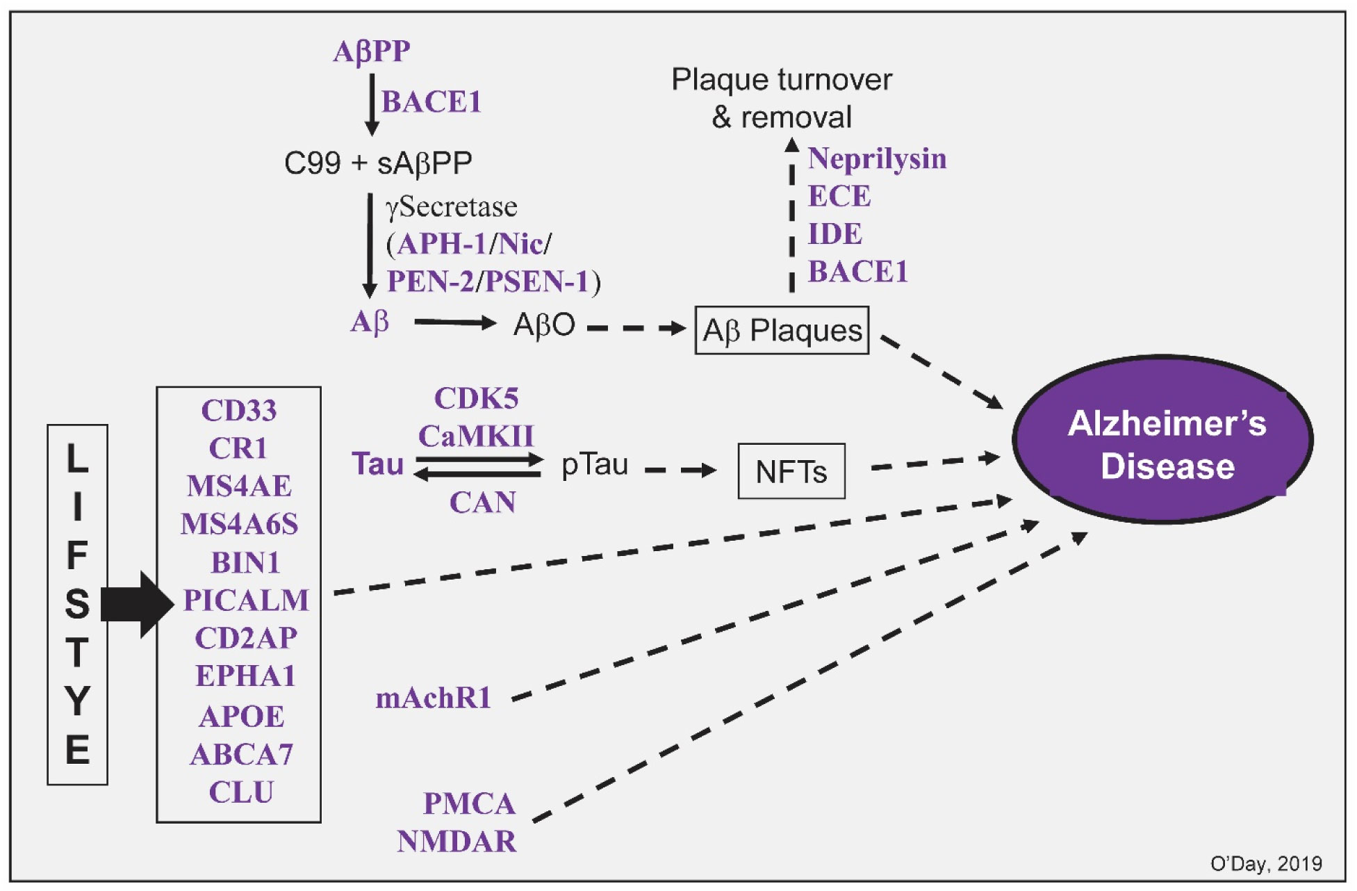
    [4] O'Day DH, Myre MA (2004) Calmodulin-binding domains in Alzheimer's disease proteins: extending the calcium hypothesis. Biochem Biophys Res Commun 230: 1051–1054.
    [5] Brini M, Cali T, Ottolini D, et al. (2014) Neuronal calcium signaling: function and dysfunction. Cell Mol Life Sci 71: 2787–2814. doi: 10.1007/s00018-013-1550-7
    [6] Berridge MJ (2010) Calcium hypothesis of Alzheimer's disease. Pflüg Arch Eur J Phy 459: 441–449. doi: 10.1007/s00424-009-0736-1
    [7] Pepke S, Kinzer-Ursem T, Mihala S, et al. (2010) A dynamic model of interactions of Ca2+, calmodulin, and catalytic subunits of Ca2+/calmodulin-dependent protein kinase II. PLoS Comput Biol 6: e1000675. doi: 10.1371/journal.pcbi.1000675
    [8] 
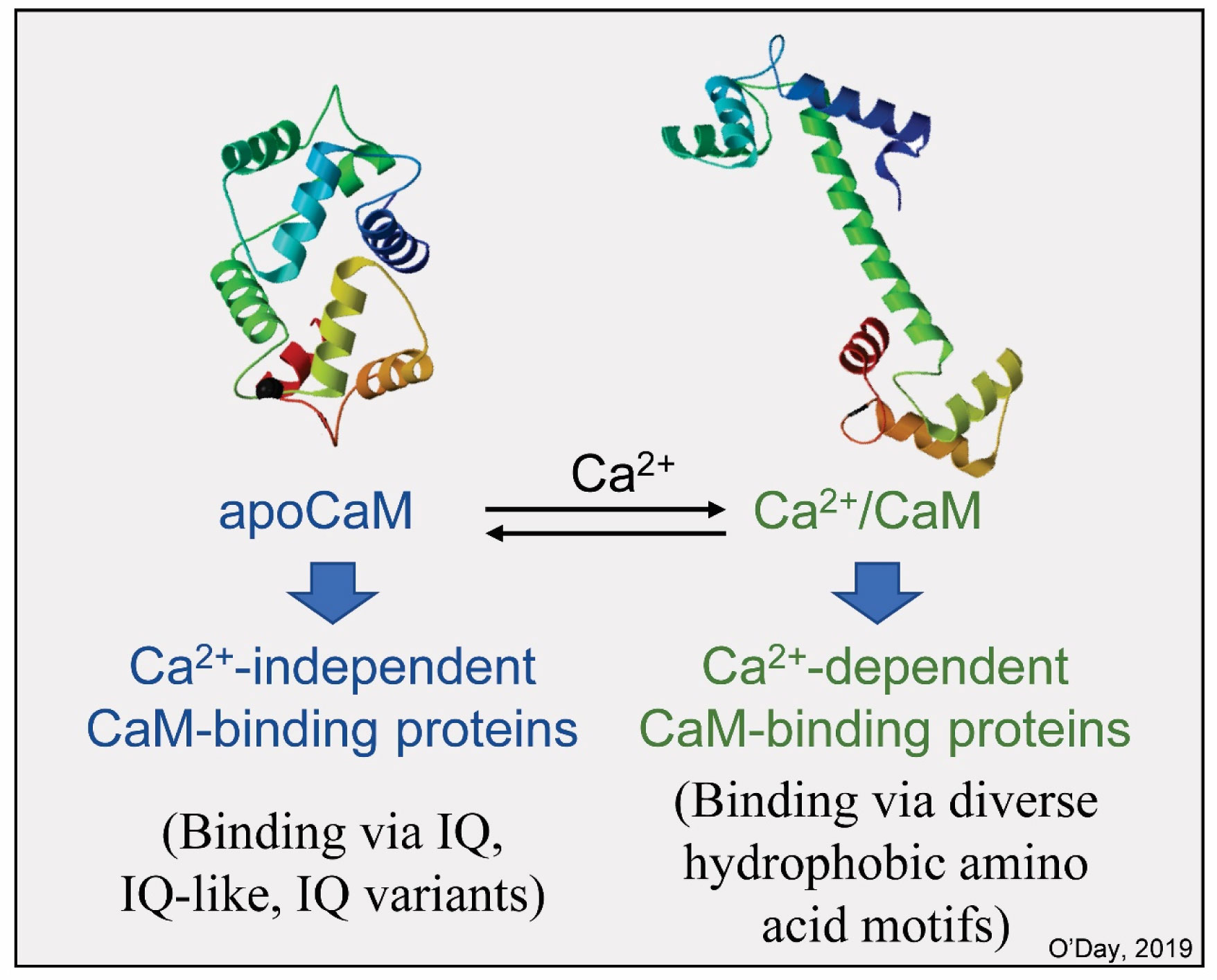
Chin D, Means AR (2000) Calmodulin: A prototypical calcium sensor. Trends Cell Biol 10: 322–328. doi: 10.1016/S0962-8924(00)01800-6
    [9] Rhoads AR, Friedberg F (1997) Sequence motifs for calmodulin recognition. FASEB J 11: 331–340. doi: 10.1096/fasebj.11.5.9141499
    [10] Tidow H, Nissen P (2013) Structural diversity of calmodulin binding to its target sites. FEBS J 280: 5551–5565. doi: 10.1111/febs.12296
    [11] Sharma RK, Parameswaran S (2018) Calmodulin-binding proteins: A journey of 40 years. Cell Calcium 75: 89–100. doi: 10.1016/j.ceca.2018.09.002
    [12] Hippius H, Neundörfer G (2003) The discovery of Alzheimer's disease. Dialogues Clin Neurosci 5: 101–108.
    [13] Myre MA, Tesco G, Tanzi RE, et al. (2005) Calmodulin binding to APP and the APLPs. Molecular Mechanisms of Neurodegeneration: A Joint Biochemical Society/Neuroscience Ireland Focused Meeting; March 13–16, University College Dublin, Republic of Ireland.
    [14] Canobbio I, Catricalà S, Balduini C, et al. (2011) Calmodulin regulates the non-amyloidogenic metabolism of amyloid precursor protein in platelets. Biochem Biophys Acta 1813: 500–506. doi: 10.1016/j.bbamcr.2010.12.002
    [15] Chavez SE, O'Day DH (2007) Calmodulin binds to and regulates the activity of beta-secretase (BACE1). Curr Res Alzheimers Dis 1: 37–47.
    [16] Corbacho I, Berrocal M, Torok K, et al. (2017) High affinity binding of amyloid β-peptide to calmodulin: Structural and functional implications. Biochem Biophys Res Commun 486: 992–997. doi: 10.1016/j.bbrc.2017.03.151
    [17] Cline EN, Bicca MA, Viola KL, et al. (2018) The amyloid-β oligomer hypothesis: Beginning of the third decade. J Alzheimers Dis 64: S567–S610. doi: 10.3233/JAD-179941
    [18] O'Day DH, Eshak K, Myre MA (2015) Calmodulin binding proteins and Alzheimer's disease: A review. J Alzheimers Dis 46: 553–569. doi: 10.3233/JAD-142772
    [19] Michno K, Knight D, Campusano JM, et al. (2009) Intracellular calcium deficits in Drosophila cholinergic neurons expressing wild type or FAD-mutant presenilin. PLoS One 4: e6904. doi: 10.1371/journal.pone.0006904
    [20] Lee YC, Wolff J (1984) Calmodulin binds to both microtubule-associated protein 2 and tau proteins. J Biol Chem 259: 1226–1230.
    [21] Padilla R, Maccioni RB, Avila J (1990) Calmodulin binds to a tubulin binding site of the microtubule-associated protein tau. Mol Cell Biochem 97: 35–41.
    [22] Huber RJ, Catalano A, O'Day DH (2013) Cyclin-dependent kinase 5 is a calmodulin-binding protein that associates with puromycin-sensitive aminopeptidase in the nucleus of Dictyostelium. Biochem Biophys Acta 1833: 11–20. doi: 10.1016/j.bbamcr.2012.10.005
    [23] Yu DY, Tong L, Song GJ, et al. (2008) Tau binds both subunits of calcineurin, and binding is impaired by calmodulin. Biochem Biophys Acta 1783: 2255–2261. doi: 10.1016/j.bbamcr.2008.06.015
    [24] Ghosh A, Geise KP (2015) Calcium/calmodulin-dependent kinase II and Alzheimer's disease. Mol Brain 8: 78. doi: 10.1186/s13041-015-0166-2
    [25] Reese LC, Taglialatela G (2011) A role for calcineurin in Alzheimer's disease. Curr Neuropharmacol 9: 685–692. doi: 10.2174/157015911798376316
    [26] Karch CM, Goate AM (2015) Alzheimer's disease risk genes and mechanisms of disease pathogenesis. Biol Psych 77: 43–51. doi: 10.1016/j.biopsych.2014.05.006
    [27] Newcombe EA Camats-Perna J, Silva ML, et al. (2018) Inflammation: The link between comorbidities, genetics and Alzheimer's disease. J Neuroinflamm 15: 276. doi: 10.1186/s12974-018-1313-3
    [28] Di Batista AM, Heinsinger NM, Rebeck GW (2016) Alzheimer's disease genetic risk factor APOE-4 also affects normal brain function. Curr Alzheimer Res 13: 1200–1207. doi: 10.2174/1567205013666160401115127
    [29] Hansen DV, Hanson JE, Sheng M (2017) Microglia in Alzheimer's disease. J Cell Biol 217: 459–172.
    [30] Navarro V, Sanchez-Mejias E, Jimenez S, et al. (2018) Microglia in Alzheimer's disease: Activated, dysfunctional or degenerative. Front Aging Neurosci 10: 140. doi: 10.3389/fnagi.2018.00140
    [31] Jiang S, Li Y, Zhang C, et al. (2014) M1 muscarinic acetylcholine receptor in Alzheimer's disease. Neurosci Bull 30: 295–307. doi: 10.1007/s12264-013-1406-z
    [32] Lucas JL, Wang D, Sadée W (2006) Calmodulin binding to peptides derived from the i3 loop of muscarinic receptors. Pharm Res 23: 647–653. doi: 10.1007/s11095-006-9784-9
    [33] Berrocal M, Sepulveda MR, Vazquez-Hernandez M, et al. (2012) Calmodulin antagonizes amyloid-β peptides-mediated inhibition of brain plasma membrane Ca2+-ATPase. Biochim Biophys Acta 1822: 961–969. doi: 10.1016/j.bbadis.2012.02.013
    [34] Ehlers MD, Zhang S, Bernhadt JP, et al. (1996) Inactivation of NMDA receptors by direct interaction of calmodulin with the NR1 subunit. Cell 84: 745–755. doi: 10.1016/S0092-8674(00)81052-1
    [35] Rycroft BK, Gibb AJ (2002) Direct effects of calmodulin on NMDA receptor single-channel gating in rat hippocampal granule cells. J Neurosci 22: 8860–8868. doi: 10.1523/JNEUROSCI.22-20-08860.2002
    [36] Wang R, Reddy PH (2017) Role of glutamate and NMDA receptors in Alzheimer's disease. J Alzheimers Dis 57: 1041–1048. doi: 10.3233/JAD-160763
    [37] Hong HS, Hwang JY, Son SM, et al. (2010) FK506 reduces amyloid plaque burden and induces MMP-9 in AβPP/PS1 double transgenic mice. J Alzheimers Dis 22: 97–105. doi: 10.3233/JAD-2010-100261
    [38] Rozkalne A, Hyman BT, Spires-Jones TL (2011) Calcineurin inhibition with FK506 ameliorates dendritic spine density deficits in plaque-bearing Alzheimer model mice. Neurobiol Dis 41: 650–654. doi: 10.1016/j.nbd.2010.11.014
    [39] Taglialatella G, Rastellini C, Cicalese L (2015) Reduced incidence of dementia in solid organ transplant patients treated with calcineurin inhibitors. J Alzheimers Dis 47: 329–333. doi: 10.3233/JAD-150065
    [40] Popugaeva E, Pchitskaya E, Bezprozvanny I (2017) Dysregulation of neuronal calcium homeostasis in Alzheimer's disease-A therapeutic opportunity? Biochem Biophys Res Commun 483: 998–1004. doi: 10.1016/j.bbrc.2016.09.053
  • Reader Comments
  • © 2019 the Author(s), licensee AIMS Press. This is an open access article distributed under the terms of the Creative Commons Attribution License (http://creativecommons.org/licenses/by/4.0)
通讯作者: 陈斌, bchen63@163.com
  • 1. 

    沈阳化工大学材料科学与工程学院 沈阳 110142

  1. 本站搜索
  2. 百度学术搜索
  3. 万方数据库搜索
  4. CNKI搜索

Metrics

Article views(6098) PDF downloads(670) Cited by(18)

Figures and Tables

Figures(2)

Other Articles By Authors

/

DownLoad:  Full-Size Img  PowerPoint
Return
Return

Catalog