Sleep impairment and work-related stress are common issues that influence employee well-being and organizational outcomes. Impaired sleep depletes cognitive and emotional resources, increasing stress and the likelihood of counterproductive work behaviors directed toward the organization (CWB-O). This cross-sectional study, guided by the conservation of resources (COR) theory, explores the relationships between impaired sleep, work-related stress, and CWB-O, considering substance use as a dysfunctional coping strategy.
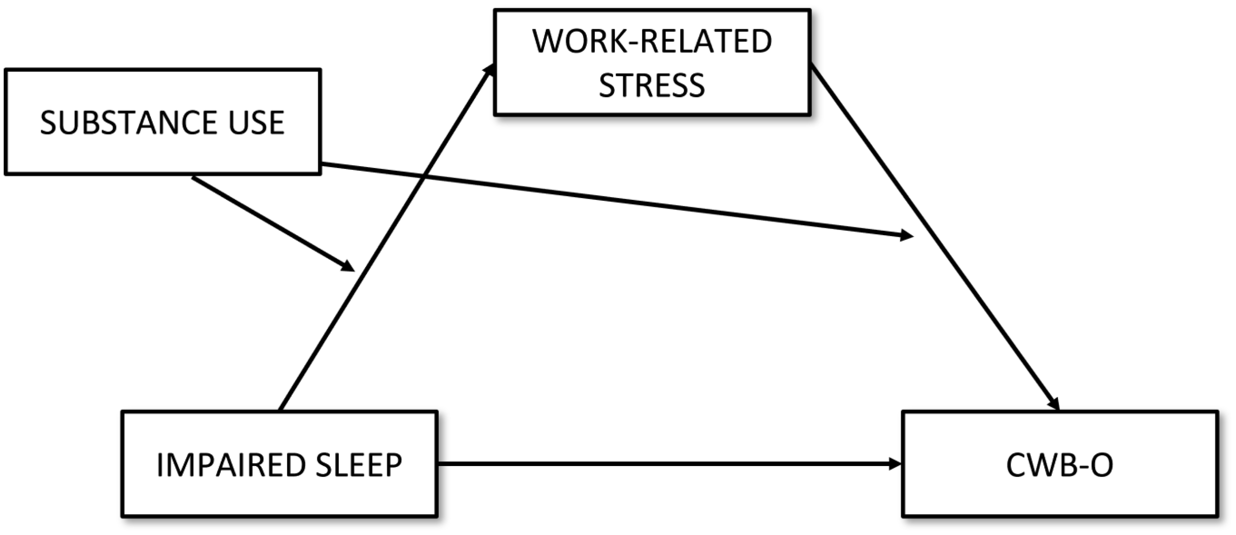
A sample of 302 Italian employees completed an online survey. Sleep impairment was assessed using the Insomnia Severity Index, work-related stress was assessed with the Perceived Stress Scale, CWB-O was assessed with the Counterproductive Work Behavior Checklist, and substance use as a coping strategy was assessed using the Brief COPE. A moderated mediation model was tested to examine the indirect effects of sleep impairment on CWB-O via work-related stress, with substance use moderating both the sleep–stress and stress–CWB-O relationships.
The results supported the hypothesis that the relationship between sleep impairment and CWB-O is mediated by work-related stress. Sleep difficulties significantly increased work-related stress, which in turn led to higher levels of CWB-O. Substance use did not moderate the relationship between sleep and work-related stress. It did, however, significantly moderate the relationship between work-related stress and CWB-O, with higher levels of substance use amplifying the impact of stress on behavioral dysregulation.
This study contributes to our understanding of how impaired sleep, work-related stress, and substance use interact to influence deviant behaviors at work. The findings align with COR theory, highlighting the role of resource depletion and dysfunctional coping in workplace behavior, and suggest that organizational interventions should also consider programs aimed at improving sleep quality and addressing substance use to reduce the likelihood of deviant behaviors at work.
Citation: Francesco Marcatto, Donatella Ferrante, Mateusz Paliga, Edanur Kanbur, Nicola Magnavita. Behavioral dysregulation at work: A moderated mediation analysis of sleep impairment, work-related stress, and substance use[J]. AIMS Public Health, 2025, 12(2): 290-309. doi: 10.3934/publichealth.2025018
Sleep impairment and work-related stress are common issues that influence employee well-being and organizational outcomes. Impaired sleep depletes cognitive and emotional resources, increasing stress and the likelihood of counterproductive work behaviors directed toward the organization (CWB-O). This cross-sectional study, guided by the conservation of resources (COR) theory, explores the relationships between impaired sleep, work-related stress, and CWB-O, considering substance use as a dysfunctional coping strategy.
A sample of 302 Italian employees completed an online survey. Sleep impairment was assessed using the Insomnia Severity Index, work-related stress was assessed with the Perceived Stress Scale, CWB-O was assessed with the Counterproductive Work Behavior Checklist, and substance use as a coping strategy was assessed using the Brief COPE. A moderated mediation model was tested to examine the indirect effects of sleep impairment on CWB-O via work-related stress, with substance use moderating both the sleep–stress and stress–CWB-O relationships.
The results supported the hypothesis that the relationship between sleep impairment and CWB-O is mediated by work-related stress. Sleep difficulties significantly increased work-related stress, which in turn led to higher levels of CWB-O. Substance use did not moderate the relationship between sleep and work-related stress. It did, however, significantly moderate the relationship between work-related stress and CWB-O, with higher levels of substance use amplifying the impact of stress on behavioral dysregulation.
This study contributes to our understanding of how impaired sleep, work-related stress, and substance use interact to influence deviant behaviors at work. The findings align with COR theory, highlighting the role of resource depletion and dysfunctional coping in workplace behavior, and suggest that organizational interventions should also consider programs aimed at improving sleep quality and addressing substance use to reduce the likelihood of deviant behaviors at work.

| [1] | European Foundation for the Improvement of Living and Working Conditions. Work organisation. [cited 2024 Dec 08th] Available from: https://www.eurofound.europa.eu/en/topic/work-organisation |
| [2] |
Wilson MG, Dejoy DM, Vandenberg RJ, et al. (2004) Work characteristics and employee health and well-being: Test of a model of healthy work organization. J Occup Organ Psychol 77: 565-588. https://doi.org/10.1348/0963179042596522 
|
| [3] |
Di Fabio A (2017) Positive Healthy Organizations: Promoting Well-Being, Meaningfulness, and Sustainability in Organizations. Front Psychol 8: 1938. https://doi.org/10.3389/fpsyg.2017.01938
|
| [4] | Elovainio M, Heponiemi T, Sinervo T, et al. (2010) Organizational justice and health; review of evidence. G Ital Med Lav Ergon 32: B5-B9. |
| [5] |
Magnavita N, Chiorri C, Acquadro Maran D, et al. (2022) Organizational Justice and Health: A Survey in Hospital Workers. Int J Environ Res Public Health 19: 9739. https://doi.org/10.3390/ijerph19159739
|
| [6] |
Magnavita N, Chiorri C, Karimi L, et al. (2022) The Impact of Quality of Work Organization on Distress and Absenteeism among Healthcare Workers. Int J Environ Res Public Health 19: 13458. https://doi.org/10.3390/ijerph192013458
|
| [7] |
Whitford AB, Lee SY, Yun T, et al. (2010) Collaborative Behavior and the Performance of Government Agencies. Int Public Manag J 13: 321-349. https://doi.org/10.1080/10967494.2010.529378
|
| [8] |
Fleming AC, O'Brien K, Steele S, et al. (2022) An investigation of the nature and consequences of counterproductive work behavior. Hum Perform 35: 178-192. https://doi.org/10.1080/08959285.2022.2102635
|
| [9] | Spector PE, Fox S (2002) An emotion-centered model of voluntary work behavior: Some parallels between counterproductive work behavior and organizational citizenship behavior. Hum Resour Manag Rev 12: 269-292. https://doi.org/10.1016/S1053-4822(02)00049-9 |
| [10] |
De Clercq D, Haq IU, Azeem MU (2019) Time-related work stress and counterproductive work behavior. Pers Rev 48: 1756-1781. https://doi.org/10.1108/PR-07-2018-0241
|
| [11] |
Lehman WE, Simpson DD (1992) Employee substance use and on-the-job behaviors. J Appl Psychol 77: 309-321. https://psycnet.apa.org/doi/10.1037/0021-9010.77.3.309
|
| [12] |
Garbarino S, Lanteri P, Durando P, et al. (2016) Co-Morbidity, Mortality, Quality of Life and the Healthcare/Welfare/Social Costs of Disordered Sleep: A Rapid Review. Int J Environ Res Public Health 13: 831. https://doi.org/10.3390/ijerph13080831
|
| [13] |
Magnavita N, Garbarino S (2017) Sleep, Health and Wellness at Work: A Scoping Review. Int J Environ Res Public Health 14: 1347. https://doi.org/10.3390/ijerph14111347
|
| [14] |
Garbarino S, Guglielmi O, Sanna A, et al. (2016) Risk of Occupational Accidents in Workers with Obstructive Sleep Apnea: Systematic Review and Meta-analysis. Sleep 39: 1211-1218. https://doi.org/10.5665/sleep.5834
|
| [15] |
Garbarino S, Magnavita N, Guglielmi O, et al. (2017) Insomnia is associated with road accidents. Further evidence from a study on truck drivers. PLoS One 12: e0187256. https://doi.org/10.1371/journal.pone.0187256
|
| [16] |
Chang AM, Aeschbach D, Duffy JF, et al. (2015) Evening use of light-emitting eReaders negatively affects sleep, circadian timing, and next-morning alertness. Proc Natl Acad Sci 112: 1232-1237. https://doi.org/10.1073/pnas.1418490112
|
| [17] |
Dawson D, Encel N, Lushington K (1995) Improving Adaptation to Simulated Night Shift: Timed Exposure to Bright Light Versus Daytime Melatonin Administration. Sleep 18: 11-21. https://doi.org/10.1093/sleep/18.1.11
|
| [18] |
LeBlanc M, Mérette C, Savard J, et al. (2009) Incidence and Risk Factors of Insomnia in a Population-Based Sample. Sleep 32: 1027-1037. https://doi.org/10.1093/sleep/32.8.1027
|
| [19] |
Fietze I, Rosenblum L, Salanitro M, et al. (2022) The Interplay Between Poor Sleep and Work-Related Health. Front Public Health 10. https://doi.org/10.3389/fpubh.2022.866750
|
| [20] |
Swanson LM, Arnedt JT, Rosekind MR, et al. (2011) Sleep disorders and work performance: findings from the 2008 National Sleep Foundation Sleep in America poll. J Sleep Res 20: 487-494. https://doi.org/10.1111/j.1365-2869.2010.00890.x
|
| [21] |
Van Laethem M, Beckers DGJ, Kompier MAJ, et al. (2015) Bidirectional relations between work-related stress, sleep quality and perseverative cognition. J Psychosom Res 79: 391-398. https://doi.org/10.1016/j.jpsychores.2015.08.011
|
| [22] | Magnavita N, Chirico F, Garbarino S, et al. (2024) Stress, sleep, and cardiovascular risk in police officers: A scoping review. J Health Soc Sci 9: 9-23. https://dx.doi.org/10.19204/2024/STRS1 |
| [23] |
Garbarino S, Durando P, Guglielmi O, et al. (2016) Sleep Apnea, Sleep Debt and Daytime Sleepiness Are Independently Associated with Road Accidents. A Cross-Sectional Study on Truck Drivers. PLoS One 11: e0166262. https://doi.org/10.1371/journal.pone.0166262
|
| [24] |
Qiu D, Li Y, Li R, et al. (2022) Long working hours, work-related stressors and sleep disturbances among Chinese government employees: A large population-based follow-up study. Sleep Med 96: 79-86. https://doi.org/10.1016/j.sleep.2022.05.005
|
| [25] |
Barnes CM, Guarana C, Lee J, et al. (2023) Using wearable technology (closed loop acoustic stimulation) to improve sleep quality and work outcomes. J Appl Psychol 108: 1391-1407. https://psycnet.apa.org/doi/10.1037/apl0001077
|
| [26] |
Killgore WDS (2010) Effects of sleep deprivation on cognition. Progress in Brain Research . Elsevier 105-129. https://doi.org/10.1016/B978-0-444-53702-7.00007-5
|
| [27] |
Walker MP (2009) The Role of Sleep in Cognition and Emotion. Ann N Y Acad Sci 1156: 168-197. https://doi.org/10.1111/j.1749-6632.2009.04416.x
|
| [28] |
Pilcher JJ, Huffcutt AI (1996) Effects of Sleep Deprivation on Performance: A Meta-Analysis. Sleep 19: 318-326. https://doi.org/10.1093/sleep/19.4.318
|
| [29] |
Lim J, Dinges DF (2010) A meta-analysis of the impact of short-term sleep deprivation on cognitive variables. Psychol Bull 136: 375-389. https://doi.org/10.1037/a0018883
|
| [30] |
Åkerstedt T, Nordin M, Alfredsson L, et al. (2012) Predicting changes in sleep complaints from baseline values and changes in work demands, work control, and work preoccupation – The WOLF-project. Sleep Med 13: 73-80. https://doi.org/10.1016/j.sleep.2011.04.015
|
| [31] |
Kim G, Min B, Jung J, et al. (2016) The association of relational and organizational job stress factors with sleep disorder: analysis of the 3rd Korean working conditions survey (2011). Ann Occup Environ Med 28: 46. https://doi.org/10.1186/s40557-016-0131-2
|
| [32] |
Levi L (1990) Occupational stress: Spice of life or kiss of death?. Am Psychol 45: 1142-1145. https://psycnet.apa.org/doi/10.1037/0003-066X.45.10.1142
|
| [33] |
Maslach C, Schaufeli WB, Leiter MP (2001) Job Burnout. Annu Rev Psychol 52: 397-422. https://doi.org/10.1146/annurev.psych.52.1.397
|
| [34] |
Podsakoff NP, LePine JA, LePine MA (2007) Differential challenge stressor-hindrance stressor relationships with job attitudes, turnover intentions, turnover, and withdrawal behavior: A meta-analysis. J Appl Psychol 92: 438-454. https://psycnet.apa.org/doi/10.1037/0021-9010.92.2.438
|
| [35] |
Guglielmi O, Magnavita N, Garbarino S (2018) Sleep quality, obstructive sleep apnea, and psychological distress in truck drivers: a cross-sectional study. Soc Psychiatry Psychiatr Epidemiol 53: 531-536. https://doi.org/10.1007/s00127-017-1474-x
|
| [36] |
Magnavita N, Capitanelli I, Garbarino S, et al. (2018) Work-related stress as a cardiovascular risk factor in police officers: a systematic review of evidence. Int Arch Occup Environ Health 91: 377-389. https://doi.org/10.1007/s00420-018-1290-y
|
| [37] |
Marcatto F, Ferrante D (2021) Beyond the assessment of work-related stress risk: the management standards approach for organizational wellbeing. G Ital Med Lav Ergon 43: 126-130.
|
| [38] |
Marcatto F, Patriarca E, Bramuzzo D, et al. (2024) Job demands and DHEA-S levels: a study on healthcare workers. Occup Med 74: 225-229. https://doi.org/10.1093/occmed/kqae017
|
| [39] |
Acquadro Maran D, Magnavita N, Garbarino S (2022) Identifying Organizational Stressors That Could Be a Source of Discomfort in Police Officers: A Thematic Review. Int J Environ Res Public Health 19: 3720. https://doi.org/10.3390/ijerph19063720
|
| [40] |
Rees G (2020) Getting the Sergeants on your side: the importance of interpersonal relationships and cultural interoperability for generating interagency collaboration between nurses and the police in custody suites. Sociol Health Illn 42: 111-125. https://doi.org/10.1111/1467-9566.12989
|
| [41] |
Magnavita N (2014) Workplace violence and occupational stress in healthcare workers: a chicken-and-egg situation-results of a 6-year follow-up study. J Nurs Scholarsh 46: 366-376. https://doi.org/10.1111/jnu.12088
|
| [42] |
Magnavita N (2013) The exploding spark: workplace violence in an infectious disease hospital--a longitudinal study. BioMed Res Int 2013: 316358. https://doi.org/10.1155/2013/316358
|
| [43] |
Marcatto F, Orrico K, Luis O, et al. (2021) Exposure to organizational stressors and health outcomes in a sample of Italian local police officers. Polic J Policy Pract 15: 2241-2251. https://doi.org/10.1093/police/paab052
|
| [44] |
Kim H, Kim B, Min K, et al. (2011) Association between Job Stress and Insomnia in Korean Workers. J Occup Health 53: 164-174. https://doi.org/10.1539/joh.10-0032-OA
|
| [45] |
Linton SJ (2004) Does work stress predict insomnia? A prospective study. Br J Health Psychol 9: 127-136. https://doi.org/10.1348/135910704773891005
|
| [46] |
Åkerstedt T (2006) Psychosocial stress and impaired sleep. Scand J Work Environ Health 32: 493-501. https://doi.org/10.5271/sjweh.1054
|
| [47] |
Sonnentag S, Binnewies C, Mojza EJ (2008) ‘Did you have a nice evening?’ A day-level study on recovery experiences, sleep, and affect. J Appl Psychol 93: 674-684. https://psycnet.apa.org/doi/10.1037/0021-9010.93.3.674
|
| [48] |
Garbarino S, Magnavita N (2019) Sleep problems are a strong predictor of stress-related metabolic changes in police officers. A prospective study. PLoS One 14: e0224259. https://doi.org/10.1371/journal.pone.0224259
|
| [49] |
Törnroos M, Hakulinen C, Hintsanen M, et al. (2017) Reciprocal relationships between psychosocial work characteristics and sleep problems: A two-wave study. Work Stress 31: 63-81. https://doi.org/10.1080/02678373.2017.1297968
|
| [50] |
Roehrs T, Roth T (2008) Caffeine: Sleep and daytime sleepiness. Sleep Med Rev 12: 153-162. https://doi.org/10.1016/j.smrv.2007.07.004
|
| [51] |
Crain TL, Hammer LB, Bodner T, et al. (2014) Work–family conflict, family-supportive supervisor behaviors (FSSB), and sleep outcomes. J Occup Health Psychol 19: 155-167. https://doi.org/10.1037/a0036010
|
| [52] |
Spector PE, Fox S (2005) The Stressor-Emotion Model of Counterproductive Work Behavior. Counterproductive work behavior: Investigations of actors and targets . Washington DC, US: American Psychological Association 151-174. https://psycnet.apa.org/doi/10.1037/10893-007
|
| [53] |
Christian MS, Ellis APJ (2011) Examining the Effects of Sleep Deprivation on Workplace Deviance: A Self-Regulatory Perspective. Acad Manage J 54: 913-934. https://doi.org/10.5465/amj.2010.0179
|
| [54] |
Barnes CM, Wagner DT (2009) Changing to daylight saving time cuts into sleep and increases workplace injuries. J Appl Psychol 94: 1305-1317. https://doi.org/10.1037/a0015320
|
| [55] |
Frone MR (2015) Relations of negative and positive work experiences to employee alcohol use: Testing the intervening role of negative and positive work rumination. J Occup Health Psychol 20: 148-160. https://doi.org/10.1037/a0038375
|
| [56] |
Krischer MM, Penney LM, Hunter EM (2010) Can counterproductive work behaviors be productive? CWB as emotion-focused coping. J Occup Health Psychol 15: 154-166. https://psycnet.apa.org/doi/10.1037/a0018349
|
| [57] |
Hobfoll SE (1989) Conservation of resources: A new attempt at conceptualizing stress. Am Psychol 44: 513-524. https://doi.org/10.1037//0003-066x.44.3.513
|
| [58] |
Hobfoll SE, Halbesleben J, Neveu JP, et al. (2018) Conservation of Resources in the Organizational Context: The Reality of Resources and Their Consequences. Annu Rev Organ Psychol Organ Behav 5: 103-128. https://doi.org/10.1146/annurev-orgpsych-032117-104640
|
| [59] |
Heydarifard Z, Krasikova DV (2023) Losing sleep over speaking up at work: A daily study of voice and insomnia. J Appl Psychol 108: 1559-1572. https://doi.org/10.1037/apl0001087
|
| [60] | Hobfoll SE, Shirom A (2001) Conservation of resources theory: Applications to stress and management in the workplace. Handbook of organizational behavior . New York, NY, US: Marcel Dekker 57-80. |
| [61] |
Henderson AA, Horan KA (2021) A meta-analysis of sleep and work performance: An examination of moderators and mediators. J Organ Behav 42: 1-19. https://doi.org/10.1002/job.2486
|
| [62] |
Hobfoll SE (2001) The Influence of Culture, Community, and the Nested-Self in the Stress Process: Advancing Conservation of Resources Theory. Appl Psychol 50: 337-421. https://doi.org/10.1111/1464-0597.00062
|
| [63] |
Kuper LE, Gallop R, Greenfield SF (2010) Changes in Coping Moderate Substance Abuse Outcomes Differentially across Behavioral Treatment Modality. Am J Addict 19: 543-549. https://doi.org/10.1111/j.1521-0391.2010.00074.x
|
| [64] |
Wills TA (1990) Stress and coping factors in the epidemiology of substance use. Research advances in alcohol and drug problems . New York, NY, US: Plenum Press 215-250. https://doi.org/10.1007/978-1-4899-1669-3_7
|
| [65] |
Mauro PM, Canham SL, Martins SS, et al. (2015) Substance-use coping and self-rated health among US middle-aged and older adults. Addict Behav 42: 96-100. https://doi.org/10.1016/j.addbeh.2014.10.031
|
| [66] |
Jeong J, Lee JH, Karau SJ (2024) Sleepless nights at work: examining the mediating role of insomnia in customer mistreatment. Balt J Manag 19: 308-326. https://doi.org/10.1108/BJM-11-2023-0426
|
| [67] |
Walker MP (2008) Cognitive consequences of sleep and sleep loss. Sleep Med 9: S29-S34. https://doi.org/10.1016/S1389-9457(08)70014-5
|
| [68] |
Opoku MA, Kang SW, Kim N (2023) Sleep-deprived and emotionally exhausted: depleted resources as inhibitors of creativity at work. Pers Rev 52: 1437-1461. https://doi.org/10.1108/PR-09-2021-0620
|
| [69] |
Dahlgren A, Kecklund G, Åkerstedt T (2005) Different levels of work-related stress and the effects on sleep, fatigue and cortisol. Scand J Work Environ Health 31: 277-285. https://psycnet.apa.org/doi/10.5271/sjweh.883
|
| [70] | Hobfoll SE, Freedy J (1993) Conservation of Resources: A General Stress Theory Applied To Burnout. Professional Burnout . Routledge 115-129. |
| [71] |
Opoku MA, Kang SW, Choi SB (2023) The influence of sleep on job satisfaction: examining a serial mediation model of psychological capital and burnout. Front Public Health 11: 1149367. https://doi.org/10.3389/fpubh.2023.1149367
|
| [72] |
Penney LM, Spector PE (2005) Job stress, incivility, and counterproductive work behavior (CWB): the moderating role of negative affectivity. J Organ Behav 26: 777-796. https://doi.org/10.1002/job.336
|
| [73] |
Fox S, Spector PE, Miles D (2001) Counterproductive Work Behavior (CWB) in Response to Job Stressors and Organizational Justice: Some Mediator and Moderator Tests for Autonomy and Emotions. J Vocat Behav 59: 291-309. https://doi.org/10.1006/jvbe.2001.1803
|
| [74] |
Zhao C, Zhu Y, Zhuang JY (2024) Spillover and spillback: Linking daily job insecurity to next-day counterproductive work behavior. Scand J Psychol 65: 195-205. https://doi.org/10.1111/sjop.12968
|
| [75] | Saleem F, Gopinath C (2015) Injustice, Counterproductive Work Behavior and mediating role of Work Stress. Pak J Commer Soc Sci 9: 683-699. |
| [76] |
Francis L, Barling J (2005) Organizational injustice and psychological strain. Can J Behav Sci Rev Can Sci Comport 37: 250-261. https://psycnet.apa.org/doi/10.1037/h0087260
|
| [77] |
Cohen A, Diamant A (2019) The role of justice perceptions in determining counterproductive work behaviors. Int J Hum Resour Manag 30: 2901-2924. https://doi.org/10.1080/09585192.2017.1340321
|
| [78] | Kelloway EK, Francis L, Prosser M, et al. (2010) Counterproductive work behavior as protest. Hum Resour Manag Rev 20: 18-25. https://doi.org/10.1016/j.hrmr.2009.03.014 |
| [79] |
Bakker AB, Vries JD de (2021) Job Demands–Resources theory and self-regulation: new explanations and remedies for job burnout. Anxiety Stress Coping 34: 1-21. https://doi.org/10.1080/10615806.2020.1797695
|
| [80] |
Mitchell MS, Greenbaum RL, Vogel RM, et al. (2019) Can You Handle the Pressure? The Effect of Performance Pressure on Stress Appraisals, Self-regulation, and Behavior. Acad Manage J 62: 531-552. https://doi.org/10.5465/amj.2016.0646
|
| [81] |
Johnson RE, Lin SH, Lee HW (2018) Self-Control as the Fuel for Effective Self-Regulation at Work: Antecedents, Consequences, and Boundary Conditions of Employee Self-Control. Advances in Motivation Science . Elsevier 87-128. https://doi.org/10.1016/bs.adms.2018.01.004
|
| [82] | Baqutayan SMS (2015) Stress and Coping Mechanisms: A Historical Overview. Mediterr J Soc Sci 6: 479-488. https://doi.org/10.5901/mjss.2015.v6n2s1p479 |
| [83] |
Carver CS, Scheier MF, Weintraub JK (1989) Assessing coping strategies: A theoretically based approach. J Pers Soc Psychol 56: 267-283. https://doi.org/10.1037/0022-3514.56.2.267
|
| [84] | Brady KT, Sonne SC (1999) The role of stress in alcohol use, alcoholism treatment, and relapse. Alcohol Res Health J Natl Inst Alcohol Abuse Alcohol 23: 263-271. |
| [85] |
Provencher T, Lemyre A, Vallières A, et al. (2020) Insomnia in personality disorders and substance use disorders. Curr Opin Psychol 34: 72-76. https://doi.org/10.1016/j.copsyc.2019.10.005
|
| [86] |
Taylor DJ, Bramoweth AD, Grieser EA, et al. (2013) Epidemiology of Insomnia in College Students: Relationship With Mental Health, Quality of Life, and Substance Use Difficulties. Behav Ther 44: 339-348. https://doi.org/10.1016/j.beth.2012.12.001
|
| [87] |
Angarita GA, Emadi N, Hodges S, et al. (2016) Sleep abnormalities associated with alcohol, cannabis, cocaine, and opiate use: a comprehensive review. Addict Sci Clin Pract 11: 9. https://doi.org/10.1186/s13722-016-0056-7
|
| [88] |
Chakravorty S, Vandrey RG, He S, et al. (2018) Sleep Management Among Patients with Substance Use Disorders. Med Clin North Am 102: 733-743. https://doi.org/10.1016/j.mcna.2018.02.012
|
| [89] |
Manconi M, Ferri R, Miano S, et al. (2017) Sleep architecture in insomniacs with severe benzodiazepine abuse. Clin Neurophysiol Off J Int Fed Clin Neurophysiol 128: 875-881. https://doi.org/10.1016/j.clinph.2017.03.009
|
| [90] |
Weiss NH, Kiefer R, Goncharenko S, et al. (2022) Emotion regulation and substance use: A meta-analysis. Drug Alcohol Depend 230: 109131. https://doi.org/10.1016/j.drugalcdep.2021.109131
|
| [91] |
Grant S, Contoreggi C, London ED (2000) Drug abusers show impaired performance in a laboratory test of decision making. Neuropsychologia 38: 1180-1187. https://doi.org/10.1016/S0028-3932(99)00158-X
|
| [92] |
de Wit H (2009) Impulsivity as a determinant and consequence of drug use: a review of underlying processes. Addict Biol 14: 22-31. https://doi.org/10.1111/j.1369-1600.2008.00129.x
|
| [93] |
Bastien CH, Vallières A, Morin CM (2001) Validation of the Insomnia Severity Index as an outcome measure for insomnia research. Sleep Med 2: 297-307. https://doi.org/10.1016/S1389-9457(00)00065-4
|
| [94] |
Castronovo V, Galbiati A, Marelli S, et al. (2016) Validation study of the Italian version of the Insomnia Severity Index (ISI). Neurol Sci 37: 1517-1524. https://doi.org/10.1007/s10072-016-2620-z
|
| [95] |
Marcatto F, Di Blas L, Luis O, et al. (2022) The Perceived Occupational Stress Scale: A brief tool for measuring workers' perceptions of stress at work. Eur J Psychol Assess 38: 293-306. https://psycnet.apa.org/doi/10.1027/1015-5759/a000677
|
| [96] | Barbaranelli C, Fida R, Gualandri M (2013) Assessing counterproductive work behavior: A study on the dimensionality of CWB-Checklist. TPM-Test Psychom Methodol Appl Psychol 20: 235-248. |
| [97] |
Bongelli R, Fermani A, Canestrari C, et al. (2022) Italian validation of the situational Brief Cope Scale (I-Brief Cope). PLoS One 17: e0278486. https://doi.org/10.1371/journal.pone.0278486
|
| [98] |
Wilson Van Voorhis CR, Morgan BL (2007) Understanding Power and Rules of Thumb for Determining Sample Sizes. Tutor Quant Methods Psychol 3: 43-50. https://doi.org/10.20982/tqmp.03.2.p043
|
| [99] | Kenny DA MedPower: An interactive tool for the estimation of power in tests of mediation [Computer Software] (2017). Available from: https://davidakenny.shinyapps.io/MedPower/ |
| [100] | Wills T, Shiffman S (1986) Coping and Substance Use: A Conceptual Framework. Coping and substance use . Orlando, FL: Academic Press 3-24. |


Figures(3) / Tables(4)

Francesco Marcatto, Donatella Ferrante, Mateusz Paliga, Edanur Kanbur, Nicola Magnavita. Behavioral dysregulation at work: A moderated mediation analysis of sleep impairment, work-related stress, and substance use[J]. AIMS Public Health, 2025, 12(2): 290-309. doi: 10.3934/publichealth.2025018


 DownLoad: