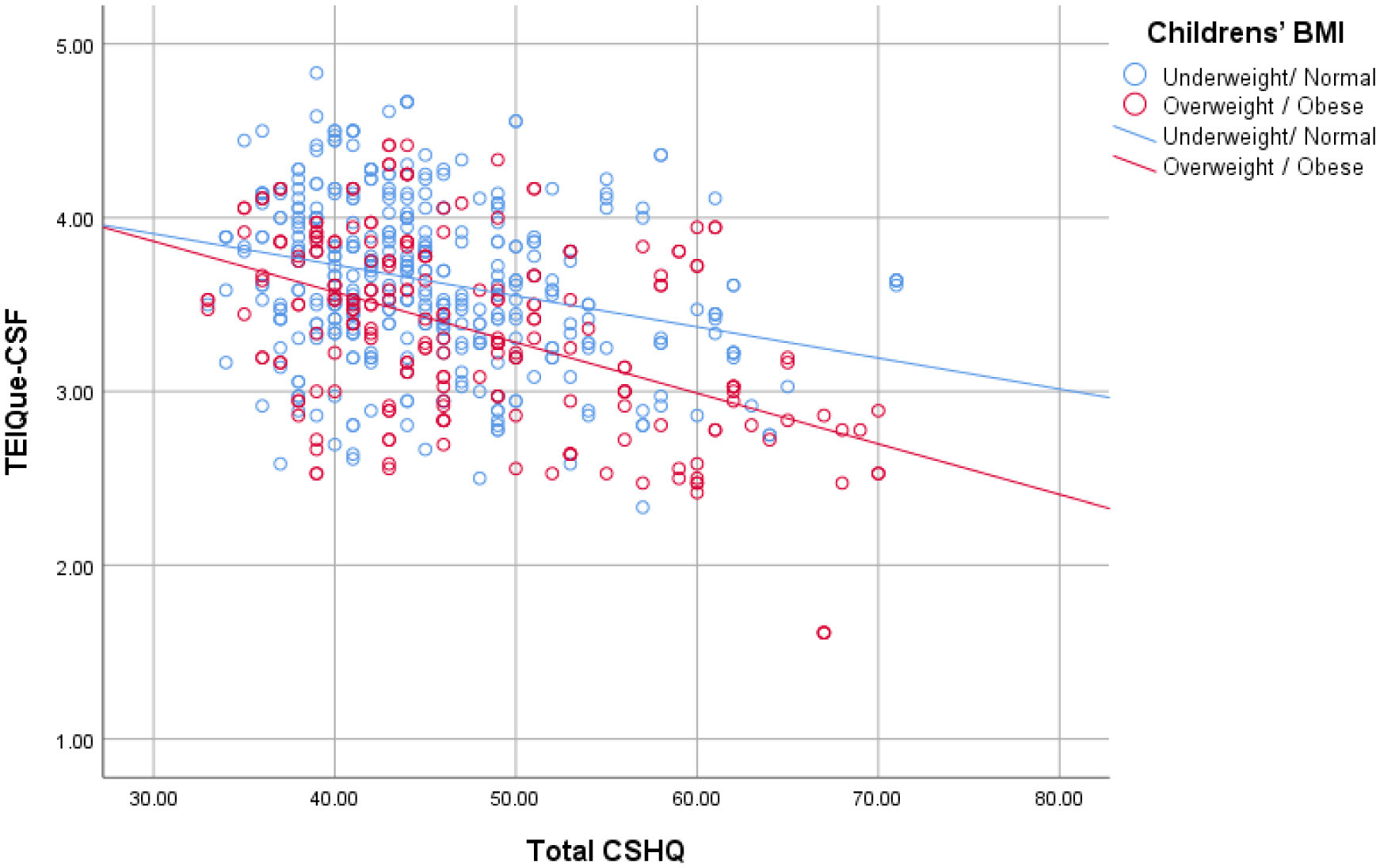
Sleep duration and quality have been increasingly recognized as critical determinants of childhood obesity risk, with insufficient sleep linked to disruptions in appetite-regulating hormones and unhealthy weight gain trajectories. Emotional intelligence, which involves recognizing, understanding, and managing one's own emotions as well as those of others, has garnered attention for its potential impact on VARIOUS aspects of health and well-being, including weight management. Moreover, childhood obesity remains a significant public health concern worldwide, with multifaceted factors contributing to its prevalence and persistence. Research is starting to reveal how sleep patterns and emotional intelligence (ΕΙ) influence children's weight status. This study aims to investigate the relationship between childhood sleep patterns, EI, and body mass index (BMI) in school-aged children. Utilizing a sample of 614 children, aged 8–12 years (mean age 10.0 y), data on emotional intelligence scores, sleep duration and quality, and BMI measurements were collected and analyzed. The results reveal significant correlations among these variables, indicating that emotional intelligence may play a crucial role in both sleep patterns and BMI outcomes in children (Mean = 3.53, SD = 0.51 in total sample; Mean = 3.53, SD = 0.51 in overweight/obese). Specifically, higher emotional intelligence scores are associated with better sleep quality and duration, as well as healthier BMI levels (p ≤ 0.001). These findings underscore the importance of considering emotional well-being and sleep hygiene in the context of childhood obesity prevention and intervention efforts. Further research is needed to elucidate the underlying mechanisms driving these relationships and to develop targeted strategies for promoting emotional intelligence and healthy sleep habits in school-aged children.
Citation: Eftychia Ferentinou, Ioannis Koutelekos, Evangelos Dousis, Eleni Evangelou, Despoina Pappa, Maria Theodoratou, Chrysoula Dafogianni. The relationship between childhood sleep, emotional intelligence and Body Mass Index in school aged children[J]. AIMS Public Health, 2025, 12(1): 77-90. doi: 10.3934/publichealth.2025006
Sleep duration and quality have been increasingly recognized as critical determinants of childhood obesity risk, with insufficient sleep linked to disruptions in appetite-regulating hormones and unhealthy weight gain trajectories. Emotional intelligence, which involves recognizing, understanding, and managing one's own emotions as well as those of others, has garnered attention for its potential impact on VARIOUS aspects of health and well-being, including weight management. Moreover, childhood obesity remains a significant public health concern worldwide, with multifaceted factors contributing to its prevalence and persistence. Research is starting to reveal how sleep patterns and emotional intelligence (ΕΙ) influence children's weight status. This study aims to investigate the relationship between childhood sleep patterns, EI, and body mass index (BMI) in school-aged children. Utilizing a sample of 614 children, aged 8–12 years (mean age 10.0 y), data on emotional intelligence scores, sleep duration and quality, and BMI measurements were collected and analyzed. The results reveal significant correlations among these variables, indicating that emotional intelligence may play a crucial role in both sleep patterns and BMI outcomes in children (Mean = 3.53, SD = 0.51 in total sample; Mean = 3.53, SD = 0.51 in overweight/obese). Specifically, higher emotional intelligence scores are associated with better sleep quality and duration, as well as healthier BMI levels (p ≤ 0.001). These findings underscore the importance of considering emotional well-being and sleep hygiene in the context of childhood obesity prevention and intervention efforts. Further research is needed to elucidate the underlying mechanisms driving these relationships and to develop targeted strategies for promoting emotional intelligence and healthy sleep habits in school-aged children.

| [1] |
Meltzer LJ, Williamson AA, Mindell JA (2021) Pediatric sleep health: It matters, and so does how we define it. Sleep Med Rev 57: 101425. https://doi.org/10.1016/j.smrv.2021.101425 
|
| [2] |
Alfano CA, Gamble AL (2009) The role of sleep in childhood psychiatric disorders. Child Youth Care Forum 38: 327-340. https://doi.org/10.1007/s10566-009-9081-y
|
| [3] |
Ong SH, Wickramaratne P, Tang M, et al. (2006) Early childhood sleep and eating problems as predictors of adolescent and adult mood and anxiety disorders. J Affect Disord 96: 1-8. https://doi.org/10.1016/j.jad.2006.05.025
|
| [4] |
Ordway MR, Condon EM, Basile Ibrahim B, et al. (2021) A systematic review of the association between sleep health and stress biomarkers in children. Sleep Med Rev 59: 101494. https://doi.org/10.1016/j.smrv.2021.101494
|
| [5] |
Gao L, Peng W, Xue H, et al. (2023) Spatial–temporal trends in global childhood overweight and obesity from 1975 to 2030: A weight mean center and projection analysis of 191 countries. Global Health 19: 53. https://doi.org/10.1186/s12992-023-00954-5
|
| [6] |
Miller AL, Miller SE, LeBourgeois MK, et al. (2019) Sleep duration and quality are associated with eating behavior in low-income toddlers. Appetite 135: 100-107. https://doi.org/10.1016/j.appet.2019.01.006
|
| [7] |
Miller AL, Lumeng JC (2016) Pathways of association from stress to obesity in early childhood. Obesity 26: 1117-1124. https://doi.org/10.1002/oby.22155
|
| [8] |
Pervanidou P, Chrousos GP (2016) Stress and pediatric obesity: Neurobiology and behavior. Fam Relat 65: 85-93. https://doi.org/10.1111/fare.12181
|
| [9] |
Lucassen EA, Cizza G (2012) The hypothalamic-pituitary-adrenal axis, obesity, and chronic stress exposure: Sleep and the HPA axis in obesity. Curr Obes Rep 1: 208-215. https://doi.org/10.1007/s13679-012-0028-5
|
| [10] |
Caliendo M, Lanzara V, Vetri L, et al. (2020) Emotional-behavioral disorders in healthy siblings of children with neurodevelopmental disorders. Medicina 56: 491. https://doi.org/10.3390/medicina56100491
|
| [11] |
Voci A, Bruni O, Ferilli MAN, et al. (2021) Sleep disorders in pediatric migraine: A questionnaire-based study. J Clin Med 10: 3575. https://doi.org/10.3390/jcm10163575
|
| [12] | Keefer KV, Saklofske D, Parker JDA (2018) Emotional intelligence, stress and health: When the going gets tough, the tough turn to emotions. An Introduction to Emotional Intelligence . Chichester: Wiley 161-183. https://doi.org/10.1002/9781394260157.ch11 |
| [13] |
Cole TJ, Flegal KM, Nicholls D, et al. (2007) Body mass index cut offs to define thinness in children and adolescents: International survey. BMJ 335: 194. https://doi.org/10.1136/bmj.39238.399444.55
|
| [14] |
Currie C, Molcho M, Boyce W, et al. (2008) Researching health inequalities in adolescents: The development of the Health Behaviour in School-aged Children (HBSC) family affluence scale. Soc Sci Med 66: 1429-1436. https://doi.org/10.1016/j.socscimed.2007.11.024
|
| [15] |
Mavroveli S, Petrides KV, Shove C, et al. (2008) Investigation of the construct of trait emotional intelligence in children. Eur Child Adolesc Psychiatry 17: 516-526. https://doi.org/10.1007/s00787-008-0696-6
|
| [16] |
Kotsou I, Nelis D, Gregoire J, et al. (2011) Emotional plasticity: Conditions and effects of improving emotional competence in adulthood. J Appl Psychol 96: 827-839. https://doi.org/10.1037/a0023047
|
| [17] |
Mikolajczak M, Avalosse H, Vancorenland S, et al. (2015) A nationally representative study of emotional competence and health. Emotion 15: 653. https://doi.org/10.1037/emo0000034
|
| [18] |
Lea RG, Qualter P, Davis SK, et al. (2018) Trait emotional intelligence and attentional bias for positive emotion: An eye tracking study. Pers Individ Differ 128: 88-93. https://doi.org/10.1016/j.paid.2018.02.017
|
| [19] |
Banjac S, Hull L, Petrides KV, et al. (2016) Validation of the Serbian adaptation of the Trait Emotional Intelligence Questionnaire-Child Form (TEIQue–CF). Psihologija 49: 375-392. https://doi.org/10.2298/PSI1604375B
|
| [20] |
Mavroudi A, Chrysochoou EA, Boyle RJ, et al. (2018) Validation of the children's sleep habits questionnaire in a sample of Greek children with allergic rhinitis. Allergol Immunopathol (Madr) 46: 389-393. https://doi.org/10.1016/j.aller.2017.09.016
|
| [21] |
Theodoratou M, Argyrides M (2024) Neuropsychological insights into coping strategies: Integrating theory and practice in clinical and therapeutic contexts. Psychiat Int 5: 53-73. https://doi.org/10.3390/psychiatryint5010005
|
| [22] | WHOEuropean Regional Obesity Report (2022). Available from: https://iris.who.int/bitstream/handle/10665/353747/9789289057738-eng.pdf |
| [23] |
Galván A (2020) The need for sleep in the adolescent brain. Trends Cogn Sci 24: 79-89. https://doi.org/10.1016/j.tics.2019.11.002
|
| [24] |
Hosokawa R, Tomozawa R, Fujimoto M, et al. (2022) Association between sleep habits and behavioral problems in early adolescence: A descriptive study. BMC Psychol 10: 254. https://doi.org/10.1186/s40359-022-00958-7
|
| [25] |
Hirshkowitz M, Whiton K, Albert SM, et al. (2015) National sleep foundation's sleep time duration recommendations: Methodology and results summary. Sleep Health 1: 40-43. https://doi.org/10.1016/j.sleh.2014.12.010
|
| [26] |
Owens J (2008) Classification and epidemiology of childhood sleep disorders. Prim Care Clin Office Pract 35: 533-546. https://doi.org/10.1016/j.pop.2008.06.003
|
| [27] |
Velten-Schurian K, Hautzinger M, Poets CF, et al. (2010) Association between sleep patterns and daytime functioning in children with insomnia: The contribution of parent-reported frequency of night waking and wake time after sleep onset. Sleep Med 11: 281-288. https://doi.org/10.1016/j.sleep.2009.03.012
|
| [28] |
Morrissey B, Taveras E, Allender S, et al. (2020) Sleep and obesity among children: A systematic review of multiple sleep dimensions. Pediatr Obes 15: 12619. https://doi.org/10.1111/ijpo.12619
|
| [29] |
Phu T, Doom JR (2022) Associations between cumulative risk, childhood sleep duration, and body mass index across childhood. BMC Pediatr 22: 529. https://doi.org/10.1186/s12887-022-03587-6
|
| [30] |
Herd T, King-Casas B, Kim-Spoon J (2020) Developmental changes in emotion regulation during adolescence: Associations with socioeconomic risk and family emotional context. J Youth Adolesc 49: 1545-1557. https://doi.org/10.1007/s10964-020-01193-2
|
| [31] |
Takeshima M, Ohta H, Hosoya T, et al. (2021) Association between sleep habits/disorders and emotional/behavioral problems among Japanese children. Sci Rep 11: 11438. https://doi.org/10.1038/s41598-021-91050-4
|
| [32] |
Weiss JA, Thomson K, Burnham Riosa P, et al. (2018) A randomized waitlist-controlled trial of cognitive behavior therapy to improve emotion regulation in children with autism. J Child Psychol Psychiatry 59: 1180-1191. https://doi.org/10.1111/jcpp.12915
|
| [33] |
Gruijters RJ, Raabe IJ, Hübner N (2023) Socio-emotional skills and the socioeconomic achievement gap. Sociol Educ 97: 120-147. https://doi.org/10.1177/00380407231216424
|
Figures(1) / Tables(5)

Eftychia Ferentinou, Ioannis Koutelekos, Evangelos Dousis, Eleni Evangelou, Despoina Pappa, Maria Theodoratou, Chrysoula Dafogianni. The relationship between childhood sleep, emotional intelligence and Body Mass Index in school aged children[J]. AIMS Public Health, 2025, 12(1): 77-90. doi: 10.3934/publichealth.2025006


 DownLoad: