Despite federal legislation intended to increase the prescribing of buprenorphine as medication for opioid use disorder (MOUD), such as the Drug Addiction Treatment Act (DATA) of 2000, most providers have continued to prescribe to some patients or to not prescribe at all. We aimed to determine the continuing barriers and supports needed for expanding buprenorphine prescribing and compared barriers experienced by emergency department (ED) physicians with those in other practice settings, given the unique aspects of the ED practice setting. We obtained survey data from August through November 2021 from 412 X-waivered Illinois physicians licensed to prescribe buprenorphine as MOUD, 95 (23.1%) of whom worked primarily in a hospital-based ED. Survey questions included: 1) Professional background, practice characteristics, and prescribing practices; 2) barriers to prescribing buprenorphine; 3) barriers to expanding prescribing; and 4) training/additional supports needed to facilitate buprenorphine prescribing. We used bivariate crosstabulations and multivariable OLS and binary logistic regressions to compare the responses of physicians practicing in the ED versus other practice settings and to compare physicians who prescribed buprenorphine in the past year with those who had not. There were few statistically significant differences among the examined subgroups indicating general agreement regardless of practice setting and prescribing status. The most frequently perceived barrier was having an inadequate community-based behavioral health treatment system to which OUD patients could be referred. Insurance reimbursement, difficulties building practice- and community-based systems to support buprenorphine prescribing, and challenges knowing where and how to refer patients for follow-up and ongoing support services were also prominent concerns. Based on study findings, efforts to expand buprenorphine for OUD might focus on providing support to make and manage treatment referrals and expanding the availability of community-based behavioral healthcare services. Building networks of care could potentially have a greater impact on MOUD availability than increasing the number of practitioners trained to prescribe buprenorphine.
Citation: James A. Swartz, Dana Franceschini, Nora M. Marino, Adrienne H. Call, Lisa Rosenberger, Sarah Whitehouse. Barriers and facilitators to prescribing buprenorphine for treating opioid use disorder among emergency department and other practice setting physicians[J]. AIMS Public Health, 2025, 12(1): 56-76. doi: 10.3934/publichealth.2025005
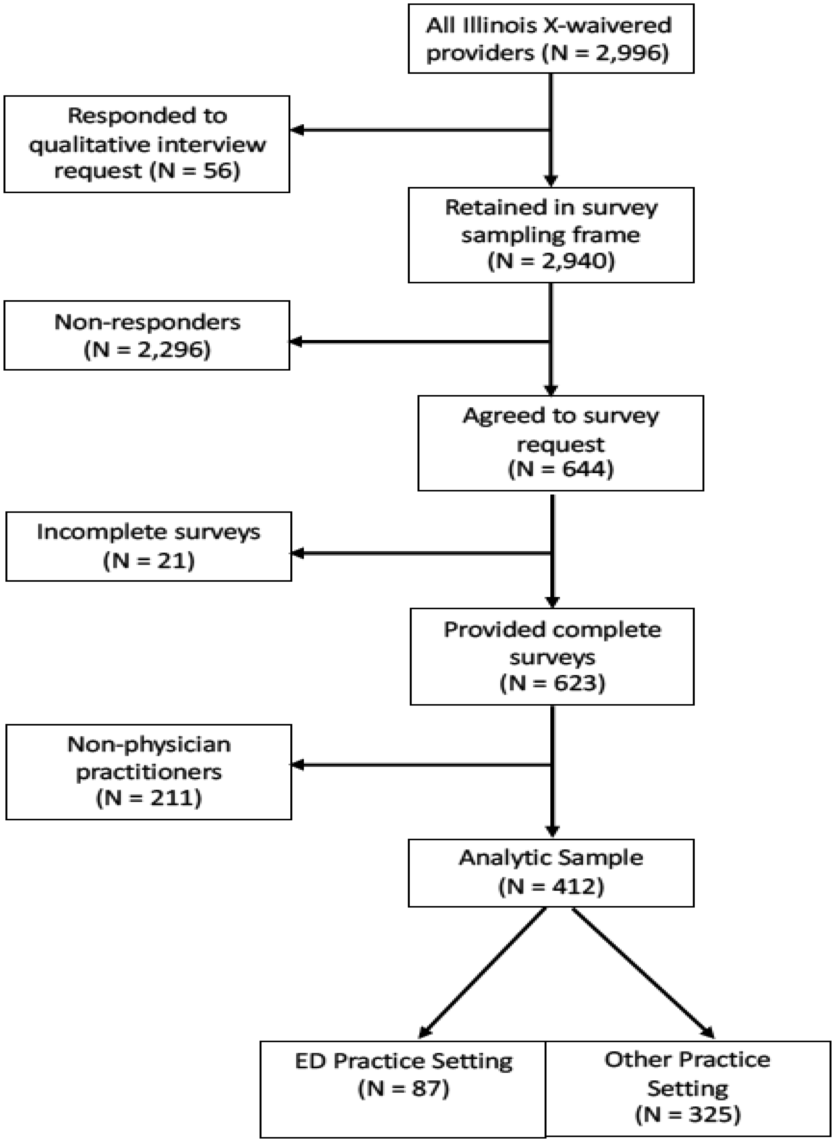
Despite federal legislation intended to increase the prescribing of buprenorphine as medication for opioid use disorder (MOUD), such as the Drug Addiction Treatment Act (DATA) of 2000, most providers have continued to prescribe to some patients or to not prescribe at all. We aimed to determine the continuing barriers and supports needed for expanding buprenorphine prescribing and compared barriers experienced by emergency department (ED) physicians with those in other practice settings, given the unique aspects of the ED practice setting. We obtained survey data from August through November 2021 from 412 X-waivered Illinois physicians licensed to prescribe buprenorphine as MOUD, 95 (23.1%) of whom worked primarily in a hospital-based ED. Survey questions included: 1) Professional background, practice characteristics, and prescribing practices; 2) barriers to prescribing buprenorphine; 3) barriers to expanding prescribing; and 4) training/additional supports needed to facilitate buprenorphine prescribing. We used bivariate crosstabulations and multivariable OLS and binary logistic regressions to compare the responses of physicians practicing in the ED versus other practice settings and to compare physicians who prescribed buprenorphine in the past year with those who had not. There were few statistically significant differences among the examined subgroups indicating general agreement regardless of practice setting and prescribing status. The most frequently perceived barrier was having an inadequate community-based behavioral health treatment system to which OUD patients could be referred. Insurance reimbursement, difficulties building practice- and community-based systems to support buprenorphine prescribing, and challenges knowing where and how to refer patients for follow-up and ongoing support services were also prominent concerns. Based on study findings, efforts to expand buprenorphine for OUD might focus on providing support to make and manage treatment referrals and expanding the availability of community-based behavioral healthcare services. Building networks of care could potentially have a greater impact on MOUD availability than increasing the number of practitioners trained to prescribe buprenorphine.

| [1] | Congressional Research ServiceThe opioid crisis in the United States: A brief history (2022). Available from: https://crsreports.congress.gov/product/pdf/IF/IF12260 |
| [2] | Drug Addiction Treatment Act of 2000, H.R. 2634, 106th Cong (2000). |
| [3] |
Saloner B, Adraka-Christou B, Stein BD, et al. (2023) Will the end of the X-waiver expand access to buprenorphine treatment achieving the full potential of the 2023 Consolidated Appropriations Act. Subst Abus 44: 108-111. https://doi.org/10.1177/08897077231186212 
|
| [4] |
McBain RK, Dick A, Sorbero M, et al. (2020) Growth and Distribution of Buprenorphine-Waivered Providers in the United States, 2007–2017. Ann Intern Med 172: 504-506. https://doi.org/10.7326/M19-2403
|
| [5] |
Larochelle MR, Jones CM, Zhang K (2023) Change in opioid and buprenorphine prescribers and prescriptions by specialty, 2016–2021. Drug Alcohol Depend 248: 109933. https://doi.org/10.1016/j.drugalcdep.2023.109933
|
| [6] |
Jones CM, Han B, Baldwin GT, et al. (2023) Use of Medication for Opioid Use Disorder Among Adults With Past-Year Opioid Use Disorder in the US, 2021. JAMA Netw Open 6: e2327488. https://doi.org/10.1001/jamanetworkopen.2023.27488
|
| [7] |
Cabreros I, Griffin BA, Saloner B, et al. (2021) Buprenorphine prescriber monthly patient caseloads: An examination of 6-year trajectories. Drug Alcohol Depend 228: 109089. https://doi.org/10.1016/j.drugalcdep.2021.109089
|
| [8] | Swartz JA, Franceschini D, Call A, et al. (2022) Substance Use Disorder Prevention that Promotes Opioid Recovery and Treatment for Patients and Communities (SUPPORT) enrolled in Illinois Medicaid managed care - final project report. Chicago, IL: Illinois Department of Healthcare and Family Services. |
| [9] |
Jones CM, Olsen Y, Ali MM, et al. (2023) Characteristics and prescribing patterns of clinicians waivered to prescribe buprenorphine for opioid use disorder before and after release of new practice guidelines. JAMA Health Forum 4: e231982. https://doi.org/10.1001/jamahealthforum.2023.1982
|
| [10] |
Thomas CP, Doyle E, Kreiner PW, et al. (2017) Prescribing patterns of buprenorphine waivered physicians. Drug Alcohol Depend 181: 213-218. https://doi.org/10.1016/j.drugalcdep.2017.10.002
|
| [11] | Pergolizzi J, LeQuang JAK, Breve F (2021) The End of the X-Waiver: Not a Moment Too Soon!. Cureus 13: e15123. https://doi.org/10.7759/cureus.15123 |
| [12] |
LeFevre N, St Louis J, Worringer E, et al. (2023) The End of the X-waiver: Excitement, Apprehension, and Opportunity. J Am Board Fam Med 36: 867-872. https://doi.org/10.3122/jabfm.2023.230048R1
|
| [13] |
Jones CM, Campopiano M, Baldwin G, et al. (2015) National and state treatment need and capacity for opioid agonist medication-assisted treatment. Am J Public Health 105: e55-e63. https://doi.org/10.2105/AJPH.2015.302664
|
| [14] |
Silwal A, Talbert J, Bohler RM, et al. (2023) State alignment with federal regulations in 2022 to relax buprenorphine 30-patient waiver requirements. Drug Alcohol Depend Rep 7: 100164. https://doi.org/10.1016/j.dadr.2023.100164
|
| [15] | Consolidated Appropriations Act, H.R. 2617 (2023). |
| [16] |
Varisco TJ, Wanat M, Hill LG, et al. (2023) The impact of the mainstreaming addiction treatment act and associated legislative action on pharmacy practice. J Am Pharm Assoc 63: 1039-1043. https://doi.org/10.1016/j.japh.2023.04.016
|
| [17] |
Cowan E, Perrone J, Bernstein SL, et al. (2023) National Institute on Drug Abuse Clinical Trials Network Meeting Report: Advancing emergency department initiation of buprenorphine for opioid use disorder. Ann Emerg Med 82: 326-335. https://doi.org/10.1016/j.annemergmed.2023.03.025
|
| [18] |
Lanham HJ, Papac J, Olmos DI, et al. (2022) Survey of barriers and facilitators to prescribing buprenorphine and clinician perceptions on the Drug Addiction Treatment Act of 2000 Waiver. JAMA Netw Open 5: e2212419. https://doi.org/10.1001/jamanetworkopen.2022.12419
|
| [19] |
Haffajee RL, Andraka-Christou B, Attermann J, et al. (2020) A mixed-method comparison of physician-reported beliefs about and barriers to treatment with medications for opioid use disorder. Subst Abuse Treat Prev Policy 15: 69. https://doi.org/10.1186/s13011-020-00312-3
|
| [20] |
Stopka TJ, Babineau DC, Gibson EB, et al. (2024) Impact of the Communities That HEAL Intervention on Buprenorphine-Waivered Practitioners and Buprenorphine Prescribing: A Prespecified Secondary Analysis of the HCS Randomized Clinical Trial. JAMA Netw Open 7: e240132. https://doi.org/10.1001/jamanetworkopen.2024.0132
|
| [21] |
Andraka-Christou B, Capone MJ (2018) A qualitative study comparing physician-reported barriers to treating addiction using buprenorphine and extended-release naltrexone in U.S. office-based practices. Int J Drug Policy 54: 9-17. https://doi.org/10.1016/j.drugpo.2017.11.021
|
| [22] |
Rhee TG, D'Onofrio G, Fiellin DA (2020) Trends in the use of buprenorphine in US emergency departments, 2002–2017. JAMA Netw Open 3: e2021209. https://doi.org/10.1001/jamanetworkopen.2020.21209
|
| [23] |
Choi S, Biello KB, Bazzi AR, et al. (2019) Age differences in emergency department utilization and repeat visits among patients with opioid use disorder at an urban safety-net hospital: A focus on young adults. Drug Alcohol Depend 200: 14-18. https://doi.org/10.1016/j.drugalcdep.2019.02.030
|
| [24] |
Kaczorowski J, Bilodeau J, A MO, et al. (2020) Emergency Department-initiated Interventions for Patients With Opioid Use Disorder: A Systematic Review. Acad Emerg Med 27: 1173-1182. https://doi.org/10.1111/acem.14054
|
| [25] |
Cao SS, Dunham SI, Simpson SA (2020) Prescribing buprenorphine for opioid use disorders in the ED: A review of best practices, barriers, and future directions. Open Access Emerg Med 12: 261-274. https://doi.org/10.2147/OAEM.S267416
|
| [26] |
Pourmand A, Beisenova K, Shukur N, et al. (2021) A practical review of buprenorphine utilization for the emergency physician in the era of decreased prescribing restrictions. Am J Emerg Med 48: 316-322. https://doi.org/10.1016/j.ajem.2021.06.065
|
| [27] |
Hawk KF, D'Onofrio G, Chawarski MC, et al. (2020) Barriers and facilitators to clinician readiness to provide emergency department-initiated buprenorphine. JAMA Netw Open 3: e204561. https://doi.org/10.1001/jamanetworkopen.2020.4561
|
| [28] |
Herring AA, Rosen AD, Samuels EA, et al. (2024) Emergency department access to buprenorphine for opioid use disorder. JAMA Netw Open 7: e2353771. https://doi.org/10.1001/jamanetworkopen.2023.53771
|
| [29] |
Kaucher KA, Caruso EH, Sungar G, et al. (2020) Evaluation of an emergency department buprenorphine induction and medication-assisted treatment referral program. Am J Emerg Med 38: 300-304. https://doi.org/10.1016/j.ajem.2019.158373
|
| [30] | SUPPORT for Patients and Communities Act, H.R. 6, 115th Cong (2018). |
| [31] | (2021) StataCorpStata 17.1 for Mac [Computer Software]. College Station, TX: StataCorp. |
| [32] |
Andrade C (2019) Multiple testing and protection against a type 1 (false positive) error using the Bonferroni and Hochberg corrections. Indian J Psychol Med 41: 99-100. https://doi.org/10.4103/IJPSYM.IJPSYM_499_18
|
| [33] | Madras B, Ahmad NJ, Wen J, et al. (2020) Improving acces to evidence-based medical treatment for opioid use disorder: Strategies to address key barriers within the treatment system. NAM Perspect 2020: 10.31478/202004b. https://doi.org/10.31478/202004b |
 publichealth-12-01-005-s001.pdf publichealth-12-01-005-s001.pdf |
 |
Figures(1) / Tables(5)

James A. Swartz, Dana Franceschini, Nora M. Marino, Adrienne H. Call, Lisa Rosenberger, Sarah Whitehouse. Barriers and facilitators to prescribing buprenorphine for treating opioid use disorder among emergency department and other practice setting physicians[J]. AIMS Public Health, 2025, 12(1): 56-76. doi: 10.3934/publichealth.2025005


 DownLoad: