In recent decades, abnormal rainfall and temperature patterns have significantly impacted the environment and human life, particularly in East Nusa Tenggara. The region is known for its low rainfall and high temperatures, making it vulnerable to drought events, which have their own complexities due to being random and changing over time. This study aimed to analyze the trend of short-term meteorological drought intensity in Timor Island, East Nusa Tenggara. The analysis was carried out by utilizing the standardized precipitation evapotranspiration index (SPEI) for a 1-month period to characterize drought in intensity, duration, and severity. A power law process approach was used to model the intensity of the event, which is inversely proportional to the magnitude of the drought event. Intensity parameters of the power law process were estimated using the maximum likelihood estimation (MLE) method to predict an increase in the intensity of drought events in the future. The probability of drought was calculated using the non-homogeneous Poisson process. The analysis showed that "extremely dry" events in Timor Island are less frequent than "very dry" and "dry" events. The power law process model's estimated intensity parameter showed a beta value greater than 1, indicating an increase in future drought events. In the next 12 months, two months of drought are expected in each region of Timor Island, East Nusa Tenggara, with the following probabilities for each region: 0.264 for Kupang City, 0.25 for Kupang, 0.265 for South Central Timor, 0.269 for North Central Timor, 0.265 for Malaka, and 0.266 for Belu. This research provides important insights into drought dynamics in vulnerable regions such as East Nusa Tenggara and its potential impact on future mitigation and adaptation planning.
Citation: Nur Hikmah Auliana, Nurtiti Sunusi, Erna Tri Herdiani. Analysis of meteorological drought periods based on the Standardized Precipitation Evapotranspiration Index (SPEI) using the Power Law Process approach[J]. AIMS Environmental Science, 2024, 11(5): 682-702. doi: 10.3934/environsci.2024034
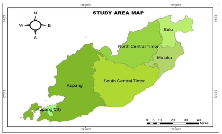
In recent decades, abnormal rainfall and temperature patterns have significantly impacted the environment and human life, particularly in East Nusa Tenggara. The region is known for its low rainfall and high temperatures, making it vulnerable to drought events, which have their own complexities due to being random and changing over time. This study aimed to analyze the trend of short-term meteorological drought intensity in Timor Island, East Nusa Tenggara. The analysis was carried out by utilizing the standardized precipitation evapotranspiration index (SPEI) for a 1-month period to characterize drought in intensity, duration, and severity. A power law process approach was used to model the intensity of the event, which is inversely proportional to the magnitude of the drought event. Intensity parameters of the power law process were estimated using the maximum likelihood estimation (MLE) method to predict an increase in the intensity of drought events in the future. The probability of drought was calculated using the non-homogeneous Poisson process. The analysis showed that "extremely dry" events in Timor Island are less frequent than "very dry" and "dry" events. The power law process model's estimated intensity parameter showed a beta value greater than 1, indicating an increase in future drought events. In the next 12 months, two months of drought are expected in each region of Timor Island, East Nusa Tenggara, with the following probabilities for each region: 0.264 for Kupang City, 0.25 for Kupang, 0.265 for South Central Timor, 0.269 for North Central Timor, 0.265 for Malaka, and 0.266 for Belu. This research provides important insights into drought dynamics in vulnerable regions such as East Nusa Tenggara and its potential impact on future mitigation and adaptation planning.

| [1] |
Hao Z, Singh VP, Xia Y (2018) Seasonal drought prediction: Advances, challenges, and future prospects. Rev Geophys 56: 108–141. https://doi.org/10.1002/2016RG000549 doi: 10.1002/2016RG000549

|
| [2] |
Sunusi N (2023) Bias of automatic weather parameter measurement in monsoon area, a case study in Makassar Coast. AIMS Environ Sci 10: 1–15. https://doi.org/10.3934/environsci.2023001 doi: 10.3934/environsci.2023001
|
| [3] |
Supari, Tangang F, Juneng L, et al. (2017) Observed changes in extreme temperature and precipitation over Indonesia. Int J Climatol 37: 1979–1997. https://doi.org/10.1002/joc.4829 doi: 10.1002/joc.4829
|
| [4] |
Easterling DR, Wallis TW, Lawrimore JH, et al. (2007) Effects of temperature and precipitation trends on US drought. Geophys Res Lett 34. https://doi.org/10.1029/2007GL031541 doi: 10.1029/2007GL031541
|
| [5] |
Yang M, Mou Y, Meng Y, et al. (2020) Modeling the effects of precipitation and temperature patterns on agricultural drought in China from 1949 to 2015. Sci Total Environ 711. https://doi.org/10.1016/j.scitotenv.2019.135139 doi: 10.1016/j.scitotenv.2019.135139
|
| [6] |
Adedeji O, Olusola A, James G, et al. (2020) Early warning systems development for agricultural drought assessment in Nigeria. Environ Monit Assess 192: 1–21. https://doi.org/10.1007/s10661-020-08730-3 doi: 10.1007/s10661-020-08730-3
|
| [7] |
Nguyen H, Thompson A, Costello C (2023) Impacts of historical droughts on maize and soybean production in the southeastern United States. Agr Water Manage 281: 1–12. https://doi.org/10.1016/j.agwat.2023.108237 doi: 10.1016/j.agwat.2023.108237
|
| [8] |
Cai S, Zuo D, Wang H, et al. (2023) Assessment of agricultural drought based on multi-source remote sensing data in a major grain producing area of Northwest China. Agr Water Manage 278: 1–17. https://doi.org/10.1016/j.agwat.2023.108142 doi: 10.1016/j.agwat.2023.108142
|
| [9] |
Yang B, Cui Q, Meng Y, et al. (2023) Combined multivariate drought index for drought assessment in China from 2003 to 2020. Agr Water Manage 281: 1–16. https://doi.org/10.1016/j.agwat.2023.108241 doi: 10.1016/j.agwat.2023.108241
|
| [10] |
Domingues LM, da Rocha HR (2022) Serial droughts and loss of hydrologic resilience in a subtropical basin: The case of water inflow into the Cantareira reservoir system in Brazil during 2013–2021. J Hydrol-Reg Stud 44: 1–18. https://doi.org/10.1016/j.ejrh.2022.101235 doi: 10.1016/j.ejrh.2022.101235
|
| [11] |
Ashraf M, Ullah K, Adnan S (2022) Satellite based impact assessment of temperature and rainfall variability on drought indices in Southern Pakistan. Int J Appl Earth Obs 108: 1–20. https://doi.org/10.1016/j.jag.2022.102726 doi: 10.1016/j.jag.2022.102726
|
| [12] |
Wilhite DA, Glantz MH (1985) Understanding: the drought phenomenon: The role of definitions. Water Int 10: 111–120. https://doi.org/10.1080/02508068508686328 doi: 10.1080/02508068508686328
|
| [13] | Palmer WC (1965) Meteorological drought. Washington DC: US Weather Bureau. |
| [14] | McKee TB, Doesken NJ, Kleist J (1993) The relationship of drought frequency and duration to time scales. 8th Conference on Applied Climatology, Anaheim, 179–184. |
| [15] |
Serrano SMV, Beguería S, Moreno JIL (2010) A multiscalar drought index sensitive to global warming: The standardized precipitation evapotranspiration index. J Climate 23: 1696–1718. https://doi.org/10.1175/2009JCLI2909.1 doi: 10.1175/2009JCLI2909.1
|
| [16] |
Clauset A, Shalizi CR, Newman ME (2009) Power-law distributions in empirical data. SIAM Rev 51: 661–703. https://doi.org/10.1137/070710111 doi: 10.1137/070710111
|
| [17] |
Rigdon SE, Basu AP (1989) The power law process: A model for the reliability of repairable systems. J Qual Technol 21: 251–260. https://doi.org/10.1080/00224065.1989.11979183 doi: 10.1080/00224065.1989.11979183
|
| [18] |
Chehade A, Shi Z, Krivtsov V (2020) Power-law nonhomogeneous Poisson process with a mixture of latent common shape parameters. Reliab Eng Syst Safe 3: 1–9. https://doi.org/10.1016/j.ress.2020.107097 doi: 10.1016/j.ress.2020.107097
|
| [19] |
Achcar JA, Rodrigues ER, Tzintzun G (2011) Using non-homogeneous Poisson models with multiple change-points to estimate the number of ozone exceedances in Mexico City. Environmetrics 22: 1–12. https://doi.org/10.1002/env.1029 doi: 10.1002/env.1029
|
| [20] |
Achcar JA, Barros EAC, Souza RMD (2016) Use of non-homogeneous Poisson process (NHPP) in presence of change-points to analyze drought periods: a case study in Brazil. Environ Ecol Stat 23: 405–419. https://doi.org/10.1007/s10651-016-0345-z doi: 10.1007/s10651-016-0345-z
|
| [21] |
Ellahi A, Hussain I, Hashmi MZ, et al. (2021) Agricultural drought periods analysis by using nonhomogeneous Poisson models and regionalization of appropriate model parameters. Tellus A 73: 1–16. http://dx.doi.org/10.1080/16000870.2021.1948241 doi: 10.1080/16000870.2021.1948241
|
| [22] |
Ghasemi P, Karbasi M, Nouri AZ, et al. (2021) Application of Gaussian process regression to forecast multi-step ahead SPEI drought index. Alex Eng J 60: 5375–5392. https://doi.org/10.1016/j.aej.2021.04.022 doi: 10.1016/j.aej.2021.04.022
|
| [23] |
Karbasi M, Karbasi M, Jamei M, et al. (2022) Development of a new wavelet-based hybrid model to forecast multi-scalar SPEI drought index (Case study: Zanjan city, Iran). Theor Appl Climatol 147: 499–522. https://doi.org/10.1007/s00704-021-03825-4 doi: 10.1007/s00704-021-03825-4
|
| [24] |
Dikshit A, Pradhan B, Huete A (2021) An improved SPEI drought forecasting approach using the long short-term memory neural network. J Environ Manage 283: 1–12. https://doi.org/10.1016/j.jenvman.2021.111979 doi: 10.1016/j.jenvman.2021.111979
|
| [25] |
Affandy NA, Anwar N, Maulana MA, et al. (2023) Forecasting meteorological drought through SPEI with SARIMA model, In AIP Conference Proceedings, 2846. http://dx.doi.org/10.1063/5.0154230 doi: 10.1063/5.0154230
|
| [26] |
Marquet PA, Quiñones RA, Abades S, et al. (2005) Scaling and power-laws in ecological systems. J Exp Biol 208: 1749–1769. http://dx.doi.org/10.1242/jeb.01588 doi: 10.1242/jeb.01588
|
| [27] |
Lyth DH, Stewart ED (1992) The curvature perturbation in power law (e.g., extended) inflation. Phys Lett B 274: 168–172. https://doi.org/10.1016/0370-2693(92)90518-9 doi: 10.1016/0370-2693(92)90518-9
|
| [28] |
Li X, Guo F, Liu YH (2021) The acceleration of charged particles and formation of power-law energy spectra in nonrelativistic magnetic reconnection. Phys Plasmas 28: 1–38. https://doi.org/10.48550/arXiv.2104.10732 doi: 10.48550/arXiv.2104.10732
|
| [29] |
Bu T, Towsley D (2002) On distinguishing between Internet power law topology generators, In Proceedings. Twenty-first annual joint conference of the ieee computer and communications societies, 2: 638–647. https://doi.org/10.1109/INFCOM.2002.1019309 doi: 10.1109/INFCOM.2002.1019309
|
| [30] |
Andreatta D, Lustres JLP, Kovalenko SA, et al. (2005) Power-law solvation dynamics in DNA over six decades in time. J Am Chem Soc 127: 7270–7271. https://doi.org/10.1021/ja044177v doi: 10.1021/ja044177v
|
| [31] | Zhao M, Xie M (1996) On maximum likelihood estimation for a general non-homogeneous Poisson process. Scand J Stat 23: 597–607. |
| [32] |
Turk LA (2014) Testing the performance of the Power Law Process model considering the use of Regression estimation approach. Int J Softw Eng Appl 5: 35–46. http://dx.doi.org/10.5121/ijsea.2014.5503 doi: 10.5121/ijsea.2014.5503
|
| [33] |
Thornthwaite CW (1948) An approach toward a rational classification of climate. Geogr Rev 38: 55–94. http://dx.doi.org/10.2307/210739 doi: 10.2307/210739
|
| [34] |
Singh VP, Guo H, Yu FX (1993) Parameter estimation for 3-parameter log-logistic distribution (LLD3) by Pome. Stoch Hydrol Hydraulics 7: 163–177. https://doi.org/10.1007/BF01585596 doi: 10.1007/BF01585596
|
| [35] | Abramowitz M, Stegun IA (1964) Handbook of mathematical functions with formulas, graphs, and mathematical tables, US Government Printing Office, 55. |
| [36] | Svoboda M, Hayes M, Wood D (2012) Standardized precipitation index: User guide. |
| [37] | Ross SM (2014) Introduction to probability models, 4 Eds., Berkeley: Academic Press, 1–647. |
| [38] |
Kuswanto H, Puspa AW, Ahmad IS, et al. (2021) Drought analysis in East Nusa Tenggara (Indonesia) using regional frequency analysis. The Scientific World J 2021: 1–10. http://dx.doi.org/10.1155/2021/6626102 doi: 10.1155/2021/6626102
|


Figures(5) / Tables(11)

Nur Hikmah Auliana, Nurtiti Sunusi, Erna Tri Herdiani. Analysis of meteorological drought periods based on the Standardized Precipitation Evapotranspiration Index (SPEI) using the Power Law Process approach[J]. AIMS Environmental Science, 2024, 11(5): 682-702. doi: 10.3934/environsci.2024034


 DownLoad: