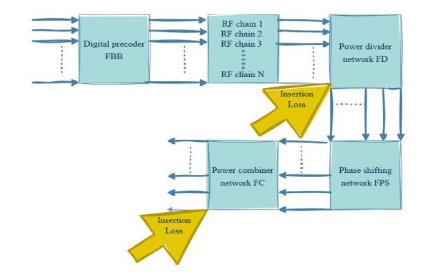
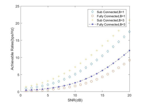
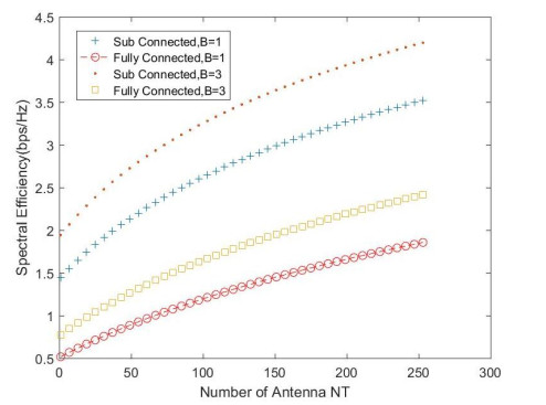
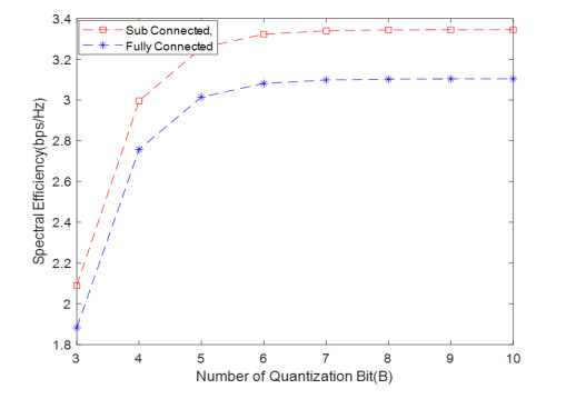
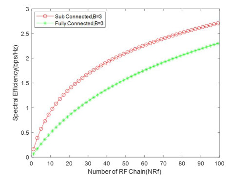
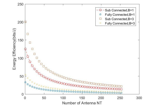
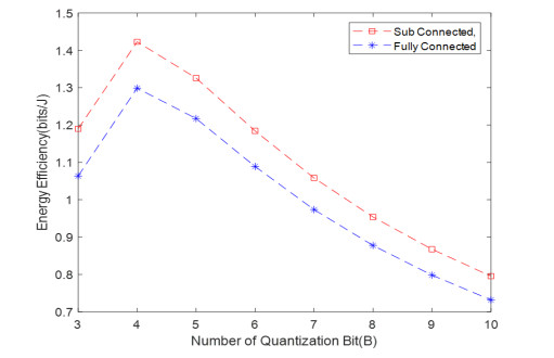
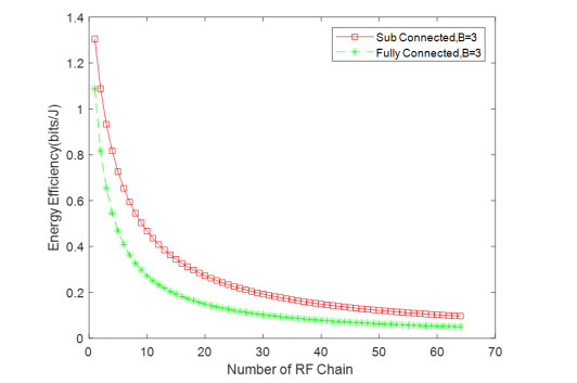
Due to an increase in the number of users and a high demand for high data rates, researchers have resorted to boosting the capacity and spectral efficiency of the next-generation wireless communication. With a limited RF chain, hybrid analog digital precoding is an appealing alternative. The hybrid precoding approach divides the beamforming process into an analog beamforming network and a digital beamforming network of a reduced size. As a result, numerous hybrid beamforming networks have been proposed. The practical effects of signal processing in the RF domain, such as the additional power loss incurred by an analog beamforming network, were not taken into account. The effectiveness of hybrid precoding structures for massive MIMO systems was examined in this study. In particular, a viable hardware network realization with insertion loss was developed. Investigating the spectral and energy efficiency of two popular hybrid precoding structures, the fully connected structure, and the subconnected structure, it was found that in a massive MIMO, the subconnected structure always performed better than the fully connected structure. Characterizing the effect of quantized analog precoding, it was shown that the subconnected structure was able to achieve better performance with fewer feedback bits than the fully connected structure.
Citation: Tadele A. Abose, Thomas O. Olwal, Muna M. Mohammed, Murad R. Hassen. Performance analysis of insertion loss incorporated hybrid precoding for massive MIMO[J]. AIMS Electronics and Electrical Engineering, 2024, 8(2): 187-210. doi: 10.3934/electreng.2024008
Due to an increase in the number of users and a high demand for high data rates, researchers have resorted to boosting the capacity and spectral efficiency of the next-generation wireless communication. With a limited RF chain, hybrid analog digital precoding is an appealing alternative. The hybrid precoding approach divides the beamforming process into an analog beamforming network and a digital beamforming network of a reduced size. As a result, numerous hybrid beamforming networks have been proposed. The practical effects of signal processing in the RF domain, such as the additional power loss incurred by an analog beamforming network, were not taken into account. The effectiveness of hybrid precoding structures for massive MIMO systems was examined in this study. In particular, a viable hardware network realization with insertion loss was developed. Investigating the spectral and energy efficiency of two popular hybrid precoding structures, the fully connected structure, and the subconnected structure, it was found that in a massive MIMO, the subconnected structure always performed better than the fully connected structure. Characterizing the effect of quantized analog precoding, it was shown that the subconnected structure was able to achieve better performance with fewer feedback bits than the fully connected structure.

| [1] |
Swindlehurst AL, Ayanoglu E, Heydari P, Capolino F (2014) Millimeter-wave massive MIMO: The next wireless revolution? IEEE Commun Mag 52: 56–62. https://doi.org/10.1109/MCOM.2014.6894453 doi: 10.1109/MCOM.2014.6894453

|
| [2] |
Karjalainen J, Nekovee M, Benn H, Kim W, Park J, Sungsoo H (2014) Challenges and Opportunities of mm-Wave Communication in 5G Networks. Proceedings of the 2014 9th International Conference on Cognitive Radio Oriented Wireless Networks and Communications (CROWNCOM), 372–376. https://doi.org/10.4108/icst.crowncom.2014.255604 doi: 10.4108/icst.crowncom.2014.255604
|
| [3] |
Marzetta TL (2010) Noncooperative cellular wireless with unlimited numbers of base station antennas. IEEE T Wirel Commun 9: 3590–3600. https://doi.org/10.1109/TWC.2010.092810.091092 doi: 10.1109/TWC.2010.092810.091092
|
| [4] |
Larsson EG, Edfors O, Tufvesson F, Marzetta TL (2014) Massive MIMO for next generation wireless systems. IEEE Commun Mag 52: 186–195. https://doi.org/10.1109/MCOM.2014.6736761 doi: 10.1109/MCOM.2014.6736761
|
| [5] |
Xie H, Wang B, Gao F, Jin S (2016) A full-space spectrum-sharing strategy for massive MIMO cognitive radio systems. IEEE J Sel Areas Commun 34: 2537–2549. https://doi.org/10.1109/JSAC.2016.2605238 doi: 10.1109/JSAC.2016.2605238
|
| [6] |
Feng W, Gao F, Shi R, Ge N, Lu J (2015) Dynamic-cell-based macro coordination for massively distributed MIMO systems. Proceedings of the 2015 IEEE Global Communications Conference (GLOBECOM), 1–6. https://doi.org/10.1109/GLOCOM.2015.7417293 doi: 10.1109/GLOCOM.2015.7417293
|
| [7] |
Ayach OE, Rajagopal S, Abu-Surra S, Pi Z, Heath RW (2014) Spatially sparse precoding in millimeter wave MIMO systems. IEEE T Wirel Commun 13: 1499–1513. https://doi.org/10.1109/TWC.2014.011714.130846 doi: 10.1109/TWC.2014.011714.130846
|
| [8] |
Roh W, Seol JY, Park J, Lee B, Lee J, Kim Y, et al. (2014) Millimeter-wave beamforming as an enabling technology for 5G cellular communications: Theoretical feasibility and prototype results. IEEE Commun Mag 52: 106–113. https://doi.org/10.1109/MCOM.2014.6736750 doi: 10.1109/MCOM.2014.6736750
|
| [9] |
Han S, Chih-Lin I, Xu Z, Rowell C (2015) Large-scale antenna systems with hybrid analog and digital beamforming for millimeter wave 5G. IEEE Commun Mag 53: 186–194. https://doi.org/10.1109/MCOM.2015.7010533 doi: 10.1109/MCOM.2015.7010533
|
| [10] |
Gao X, Dai L, Han S, Chih-Lin I, Heath RW (2016) Energy-efficient hybrid analog and digital precoding for mmwave MIMO systems with large antenna arrays. IEEE J Sel Areas Commun 34: 998–1009. https://doi.org/10.1109/JSAC.2016.2549418 doi: 10.1109/JSAC.2016.2549418
|
| [11] |
Liang L, Xu W, Dong X (2014) Low-complexity hybrid precoding in massive multiuser MIMO systems. IEEE Wireless Commun Lett 3: 653–656. https://doi.org/10.1109/LWC.2014.2363831 doi: 10.1109/LWC.2014.2363831
|
| [12] |
Wan S, Zhu H, Kang K, Qian H (2021) On the Performance of Fully-Connected and Sub-Connected Hybrid Beamforming System. IEEE T Veh Technol 70: 11078–11082. https://doi.org/10.1109/TVT.2021.3109300 doi: 10.1109/TVT.2021.3109300
|
| [13] | Ngo HQ (2015) Massive MIMO: Fundamentals and System Designs. Vol. 1642, Linköping University Electronic Press: Linköping, Sweden. https://doi.org/10.3384/lic.diva-112780 |
| [14] |
Luo Z, Luo L, Zhang X, Liu H (2022) Robust Hybrid Beamforming for Multi-user Millimeter Wave Systems with Sub-connected Structure. International Conference on Communications and Networking in China. https://doi.org/10.1007/978-3-031-34790-0_9 doi: 10.1007/978-3-031-34790-0_9
|
| [15] |
Hu Y, Qian H, Kang K, Luo X, Zhu H (2023) Joint Precoding Design for Sub-Connected Hybrid Beamforming System. IEEE T Wirel Commun. https://doi.org/10.1109/TWC.2023.3287229 doi: 10.1109/TWC.2023.3287229
|
| [16] |
Yu X, Zhang J, Letaief KB (2018) A Hardware-Efficient Analog Network Structure for Hybrid Precoding in Millimeter Wave Systems. IEEE J Sel Top Signal Process 12: 282–297. https://doi.org/10.1109/JSTSP.2018.2814009 doi: 10.1109/JSTSP.2018.2814009
|
| [17] |
Zhang Y, Du J, Chen Y, Li X, Rabie KM, Khkrel R (2020) Dual-Iterative Hybrid Beamforming Design for Millimeter-Wave Massive Multi-User MIMO Systems With Sub-Connected Structure. IEEE T Veh Technol 69: 13482–13496. https://doi.org/10.1109/TVT.2020.3029080 doi: 10.1109/TVT.2020.3029080
|
| [18] |
Garcia-Rodriguez A, Venkateswaran V, Rulikowski P, Masouros C (2016) Hybrid analog-digital precoding revisited under realistic RF modeling. IEEE Wireless Commun Lett 5: 528–531. https://doi.org/10.1109/LWC.2016.2598777 doi: 10.1109/LWC.2016.2598777
|
| [19] |
Venkateswaran V, Krishnan R (2016) Hybrid Analog and Digital Precoding: From Practical RF System Models to Information Theoretic Bounds. 2016 IEEE Globecom Workshops (GC Wkshps). https://doi.org/10.1109/GLOCOMW.2016.7848924 doi: 10.1109/GLOCOMW.2016.7848924
|
| [20] |
Song X, Kuhne T, Caire G (2019) Fully-Connected vs. Sub-Connected Hybrid Precoding Architectures for mmWave MU-MIMO. ICC 2019-2019 IEEE International Conference on Communications (ICC). https://doi.org/10.1109/ICC.2019.8761521 doi: 10.1109/ICC.2019.8761521
|
| [21] |
Ribeiro LN, Schwarz S, Rupp M, de Almeida AL (2018) Energy Efficiency of mmWave Massive MIMO Precoding with Low-Resolution DACs. IEEE Journal of Selected Topics in Signal Processing 12: 298‒312. https://doi.org/10.1109/JSTSP.2018.2824762 doi: 10.1109/JSTSP.2018.2824762
|
| [22] |
Kolawole O, Papazafeiropoulos A, Ratnarajah T (2018) Impact of Hardware Impairments on mmWave MIMO Systems with Hybrid Precoding. Proceedings of the IEEE Wireless Communication and Networking Conference. https://doi.org/10.1109/WCNC.2018.8377045 doi: 10.1109/WCNC.2018.8377045
|
| [23] |
Sheikh TA, Bora J, Hussain MA (2021) Capacity maximizing in massive MIMO with linear precoding for SSF and LSF channel with perfect CSI. Digit Commun Netw 7: 92‒99. https://doi.org/10.1016/j.dcan.2019.08.002 doi: 10.1016/j.dcan.2019.08.002
|
| [24] |
Sheikh TA, Bora J, Hussain MA (2019) Combined user and antenna selection in massive MIMO using precoding technique. International Journal of Sensors Wireless Communications and Control 9: 214‒223. https://doi.org/10.2174/2210327908666181112144939 doi: 10.2174/2210327908666181112144939
|
| [25] |
Sheikh TA, Bora J, Hussain MA (2018) Sum-rate performance of massive MIMO systems in highly scattering channel with semi-orthogonal and random user selection. Radioelectronics and Communications Systems 61: 547‒555. https://doi.org/10.3103/S0735272718120026 doi: 10.3103/S0735272718120026
|
| [26] | Papoulis A, Unnikrishna Pillai S (2012) Probability, Random Variables, and Stochastic Processes, North America: McGraw-Hill, New York, United States. |
| [27] |
Venkateswaran V, Pivit F, Guan L (2016) Hybrid RF and digital beamformer for cellular networks: Algorithms, microwave architectures, and measurements. IEEE T Microw Theory Technol 64: 2226–2243. https://doi.org/10.1109/TMTT.2016.2569583 doi: 10.1109/TMTT.2016.2569583
|
| [28] | Pozar DM (2009) Microwave Engineering, John Wiley & Sons: Hoboken, NJ, USA. |
| [29] |
Alkhateeb A, Leus G, Heath RW (2015) Limited feedback hybrid precoding for multi-user millimeter wave systems. IEEE T Wireless Commun 14: 6481–6494. https://doi.org/10.1109/TWC.2015.2455980 doi: 10.1109/TWC.2015.2455980
|
| [30] |
Fozooni M, Matthaiou M, Jin S, Alexandropoulos GC (2016) Massive MIMO relaying with hybrid processing. Proceedings of the 2016 IEEE International Conference on Communications (ICC), 1–6. https://doi.org/10.1109/ICC.2016.7510972 doi: 10.1109/ICC.2016.7510972
|
| [31] |
Du J, Xu W, Shen H, Dongy X, Zhao C (2017) Quantized Hybrid Precoding for Massive Multiuser MIMO with Insertion Loss. GLOBECOM 2017-2017 IEEE Global Communications Conference. https://doi.org/10.1109/GLOCOM.2017.8254815 doi: 10.1109/GLOCOM.2017.8254815
|
| [32] |
Du J, Xu W, Shen H, Dong X, Zhao C (2018) Hybrid Precoding Architecture for Massive Multiuser MIMO with Dissipation: Sub-Connected or Fully-Connected Structures? IEEE T Wirel Commun 17: 5465‒5479. https://doi.org/10.1109/TWC.2018.2844207 doi: 10.1109/TWC.2018.2844207
|
| [33] |
Ratnam VV, Molisch AF, Bursalioglu OY, Papadopoulos HC (2018) Hybrid beamforming with selection for multiuser massive mimo systems. IEEE T Signal Process 66: 4105–4120. https://doi.org/10.1109/TSP.2018.2838557 doi: 10.1109/TSP.2018.2838557
|
| [34] | Wei N (2007) MIMO Techniques for UTRA Long Term Evolution, Citeseer: Princeton, NJ, USA. |
| [35] |
Liu J, Bentley E (2017) Hybrid-beamforming-based millimeter-wave cellular network optimization. IEEE J Sel Area Commun 37: 2799‒2813. https://doi.org/10.23919/WIOPT.2017.7959916 doi: 10.23919/WIOPT.2017.7959916
|
| [36] |
Méndez-Rial R, Rusu C, González-Prelcic N, Alkhateeb A, Heath RW (2016) Hybrid mimo architectures for millimeter wave communications: Phase shifters or switches? IEEE Access 4: 247–267. https://doi.org/10.1109/ACCESS.2015.2514261 doi: 10.1109/ACCESS.2015.2514261
|
| [37] |
Jedda H, Ayub MM, Munir J, Mezghani A, Nossek JA (2015) Power-and spectral efficient communication system design using 1-bit quantization. Proceedings of the 2015 International Symposium on Wireless Communication Systems (ISWCS), 296–300 https://doi.org/10.1109/ISWCS.2015.7454349 doi: 10.1109/ISWCS.2015.7454349
|
| [38] |
Jing J, Xiaoxue C, Yongbin X (2016) Energy-efficiency based downlink multi-user hybrid beamforming for millimeter wave massive mimo system. J China Univ Posts Telecommun 23: 53–62. https://doi.org/10.1016/S1005-8885(16)60045-6 doi: 10.1016/S1005-8885(16)60045-6
|
| [39] |
Zhang Y, Yang Y, Dai L (2016) Energy efficiency maximization for device-to-device communication underlying cellular networks on multiple bands. IEEE Access 4: 7682–7691. https://doi.org/10.1109/ACCESS.2016.2623758 doi: 10.1109/ACCESS.2016.2623758
|
| [40] |
Abose TA, Olwal TO, Hassen MR, Bekele ES (2022) Performance Analysis and Comparisons of Hybrid Precoding Scheme for Multi-user mmWave Massive MIMO System. 2022 3rd International Conference for Emerging Technology (INCET), 1‒6. https://doi.org/10.1109/INCET54531.2022.9824401 doi: 10.1109/INCET54531.2022.9824401
|
Figures(8) / Tables(2)

Tadele A. Abose, Thomas O. Olwal, Muna M. Mohammed, Murad R. Hassen. Performance analysis of insertion loss incorporated hybrid precoding for massive MIMO[J]. AIMS Electronics and Electrical Engineering, 2024, 8(2): 187-210. doi: 10.3934/electreng.2024008


 DownLoad: