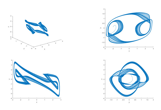
The Picard iterative approach used in the paper to derive conditions under which nonlinear ordinary differential equations based on the derivative with the Mittag-Leffler kernel admit a unique solution. Using a simple Euler approximation and Heun's approach, we solved this nonlinear equation numerically. Some examples of a nonlinear linear differential equation were considered to present the existence and uniqueness of their solutions as well as their numerical solutions. A chaotic model was also considered to show the extension of this in the case of nonlinear systems.
Citation: Abdon Atangana, Jyoti Mishra. Analysis of nonlinear ordinary differential equations with the generalized Mittag-Leffler kernel[J]. Mathematical Biosciences and Engineering, 2023, 20(11): 19763-19780. doi: 10.3934/mbe.2023875
The Picard iterative approach used in the paper to derive conditions under which nonlinear ordinary differential equations based on the derivative with the Mittag-Leffler kernel admit a unique solution. Using a simple Euler approximation and Heun's approach, we solved this nonlinear equation numerically. Some examples of a nonlinear linear differential equation were considered to present the existence and uniqueness of their solutions as well as their numerical solutions. A chaotic model was also considered to show the extension of this in the case of nonlinear systems.

| [1] |
A. Atangana, D. Baleanu, Dumitru, New fractional derivatives with nonlocal and non-singular kernel: Theory and application to heat transfer model, Thermal Sci., 20 (2016), 763–769. https://doi.org/10.2298/TSCI160111018A doi: 10.2298/TSCI160111018A

|
| [2] |
H. Khan, A. Khan, F. Jarad, A. Shah, Existence and data dependence theorems for solutions of an ABC-fractional order impulsive system, Chaos Solitons Fractals, 131 (2020), 109477. https://doi.org/10.1016/j.chaos.2019.109477 doi: 10.1016/j.chaos.2019.109477
|
| [3] |
A. Kumar, D. N. Pandey, Existence of mild solution of Atangana-Baleanu fractional differential equations with non-instantaneous impulses and with non-local conditions, Chaos Solitons Fractals, 132 (2020), 1–4. https://doi.org/10.1016/j.chaos.2019.109551 doi: 10.1016/j.chaos.2019.109551
|
| [4] |
K. Logeswari, C. Ravichandran, A new exploration on existence of fractional neutral integrodifferential equations in the concept of Atangana-Baleanu derivative, Phys. A, 544 (2020), 123454. https://doi.org/10.1016/j.physa.2019.123454 doi: 10.1016/j.physa.2019.123454
|
| [5] | R. P. Agarwal, V. Lakshmikantham, Uniqueness and Nonuniqueness Criteria for Ordinary Differential Equations, World Scientific, 2013. |
| [6] |
R. Lyons, A. S. Vatsala, R. A. Chiquet, Picard's Iterative Method for Caputo Fractional Differential Equations with Numerical Results, Mathematics, 5 (2017), 65. https://doi.org/10.3390/math5040065 doi: 10.3390/math5040065
|
| [7] | C. Arzelà, Sulle funzioni di line, Mem. Accad. Sci., 5 (1895), 55–74. |
| [8] | C. Arzelà, Un'osservazione intorno alle serie di funzioni, Tipografia Gamberini e Parmeggiani (1883), 142–159. |
| [9] | G. Ascoli, Le curve limite di una varietà data di curve, Coi tipi del Salviucci, (1884), 521–586. |
| [10] | K. A. Atkinson, An Introduction to Numerical Analysis, New York, John Wiley & Sons, 1989. |
| [11] | R. J. Barro, X. Sala-i-Martin, Growth Models with Exogenous Saving Rates, New York, McGraw-Hill, (2004), 37–51. |
| [12] | D. Acemoglu, The solow growth model, Introduction to Modern Economic Growth, Princeton University Press, (2009), 26–76. |
| [13] |
A. Khan, H. Khan, J. F. Gómez-Aguilar, T. Abdeljawad, Existence and Hyers-Ulam stability for a nonlinear singular fractional differential equations with Mittag-Leffler kernel, Chaos Solitons Fractals, 127 (2019), 422–427. https://doi.org/10.1016/j.chaos.2019.07.026 doi: 10.1016/j.chaos.2019.07.026
|
| [14] |
M. Gozen, On the existence and uniqueness of positive periodic solutions of neutral differential equations, J. Nonlinear Var. Anal., 7 (2023), 367–379. https://doi.org/10.23952/jnva.7.2023.3.03 doi: 10.23952/jnva.7.2023.3.03
|
| [15] | Uri M. Ascher, L. R. Petzold, Computer Methods for Ordinary Differential Equations and Differential-Algebraic Equations, Philadelphia: Society for Industrial and Applied Mathematics, 1998. |
| [16] | J. C. Butcher, Numerical Methods for Ordinary Differential Equations, New York, John Wiley & Sons, 2003. |
| [17] | E. Hairer, S. P. Nørsett, G. Wanner, Solving ordinary differential equations I: Nonstiff problems, Berlin, New York, Springer-Verlag, 1993. |
| [18] | Uri M. Ascher, L. R. Petzold, Computer Methods for Ordinary Differential Equations and Differential-Algebraic Equations, Philadelphia: Society for Industrial and Applied Mathematics, 1998. |


Figures(3)

Abdon Atangana, Jyoti Mishra. Analysis of nonlinear ordinary differential equations with the generalized Mittag-Leffler kernel[J]. Mathematical Biosciences and Engineering, 2023, 20(11): 19763-19780. doi: 10.3934/mbe.2023875


 DownLoad: