In this study, orange peel waste was successfully sulfonated with SO3-pyridine complex in 1-allyl-3-methylimidazolium chloride ionic liquid in various reaction conditions. 1H NMR was used to verify the occurrence of the reaction and to select the most promising material for the adsorption experiments. The degree of substitution of the sulfonated orange peel waste used for cobalt and copper removal was found to be 0.82. It was prepared with the reaction temperature and time of 70 ℃ and 60 min respectively and with the SO3-pyridine complex to-peel waste ratio of 5:1. The selected material combined with ultrafiltration removed 98% of copper and 91% of cobalt from single metal solutions and 93% of copper and 83% of cobalt from binary metal solution at pH 5 with adsorbent dosage of 12.5 mg/100 mL and initial metal concentration of 8 mg/L. Preliminary experiments were also performed with apple pomace which was sulfonated in the conditions found best for the orange peel waste. The prepared sulfonated apple pomace proved to be almost as effective in cobalt and copper removal as sulfonated orange peel waste, removing 82% of copper and 77% of cobalt from binary metal solution with 12.5 mg/100 mL dosage at pH 5 and an initial metal concentration of 8 mg/L.
Citation: Salla Kälkäjä, Lenka Breugelmans, Johanna Kärkkäinen, Katja Lappalainen. Removal of cobalt and copper from aqueous solutions with sulfonated fruit waste[J]. AIMS Materials Science, 2023, 10(5): 862-875. doi: 10.3934/matersci.2023046
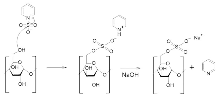
In this study, orange peel waste was successfully sulfonated with SO3-pyridine complex in 1-allyl-3-methylimidazolium chloride ionic liquid in various reaction conditions. 1H NMR was used to verify the occurrence of the reaction and to select the most promising material for the adsorption experiments. The degree of substitution of the sulfonated orange peel waste used for cobalt and copper removal was found to be 0.82. It was prepared with the reaction temperature and time of 70 ℃ and 60 min respectively and with the SO3-pyridine complex to-peel waste ratio of 5:1. The selected material combined with ultrafiltration removed 98% of copper and 91% of cobalt from single metal solutions and 93% of copper and 83% of cobalt from binary metal solution at pH 5 with adsorbent dosage of 12.5 mg/100 mL and initial metal concentration of 8 mg/L. Preliminary experiments were also performed with apple pomace which was sulfonated in the conditions found best for the orange peel waste. The prepared sulfonated apple pomace proved to be almost as effective in cobalt and copper removal as sulfonated orange peel waste, removing 82% of copper and 77% of cobalt from binary metal solution with 12.5 mg/100 mL dosage at pH 5 and an initial metal concentration of 8 mg/L.

| [1] |
Gupta A, Sharma V, Sharma K, et al. (2021) A review of adsorbents for heavy metal decontamination: Growing approach to wastewater treatment. Materials 14: 1–45. https://doi.org/10.3390/ma14164702 doi: 10.3390/ma14164702

|
| [2] |
Ali H, Khan E, Ilahi H (2019) Environmental chemistry and ecotoxicology of hazardous heavy metals: Environmental persistence, toxicity, and bioaccumulation. J Chem 2019: 6730305. https://doi.org/10.1155/2019/6730305 doi: 10.1155/2019/6730305
|
| [3] |
Qasem NAA, Mohammed RH, Lawal DU (2021) Removal of heavy metal ions from wastewater: A comprehensive and critical review. NPJ Clean Water 4: 36. https://doi.org/10.1038/s41545-021-00127-0 doi: 10.1038/s41545-021-00127-0
|
| [4] |
Chai WS, Cheun JY, Kumar PS, et al. (2021) A review on conventional and novel materials towards heavy metal adsorption in wastewater treatment application. J Clean Prod 296: 126589. https://doi.org/10.1016/j.jclepro.2021.126589 doi: 10.1016/j.jclepro.2021.126589
|
| [5] |
Wang J, Chen C (2009) Biosorbents for heavy metals removal and their future. Biotechnol Adv 27: 195–226. https://doi.org/10.1016/j.biotechadv.2008.11.002 doi: 10.1016/j.biotechadv.2008.11.002
|
| [6] |
Thakur V, Sharma E, Guleria A, et al. (2020) Modification and management of lignocellulosic waste as an ecofriendly biosorbent for the application of heavy metal ions sorption. Mater Today: Proc 32: 608–619. https://doi.org/10.1016/j.matpr.2020.02.756 doi: 10.1016/j.matpr.2020.02.756
|
| [7] |
Patel S (2012) Potential of fruit and vegetable wastes as novel biosorbents: Summarizing the recent studies. Rev Environ Sci Biotechnol 11: 365–380. https://doi.org/10.1007/S11157-012-9297-4 doi: 10.1007/S11157-012-9297-4
|
| [8] |
Jaymand M (2022) Sulfur functionality-modified starches: Review of synthesis strategies, properties, and applications. Int J Biol Macromol 197: 111–120. https://doi.org/10.1016/j.ijbiomac.2021.12.090 doi: 10.1016/j.ijbiomac.2021.12.090
|
| [9] |
Kärkkäinen J, Wik TR, Niemelä M, et al. (2016) 1H NMR-based DS determination of barley starch sulfates prepared in 1-allyl-3-methylimidazolium chloride. Carbohyd Polym 136: 721–727. https://doi.org/10.1016/j.carbpol.2015.09.097 doi: 10.1016/j.carbpol.2015.09.097
|
| [10] |
Nanda B, Sailu MS, Priyaranjan PM, et al. (2021) Green solvents: A suitable alternative for sustainable chemistry. Mater Today: Proc 47: 1234–1240. https://doi.org/10.1016/j.matpr.2021.06.458 doi: 10.1016/j.matpr.2021.06.458
|
| [11] |
Gericke M, Liebert T, Heinze T (2009) Interaction of ionic liquids with polysaccharides, 8—Synthesis of cellulose sulfates suitable for polyelectrolyte complex formation. Macromol Biosci 9: 343–353. https://doi.org/10.1002/mabi.200800329 doi: 10.1002/mabi.200800329
|
| [12] |
Qin Z, Ji L, Yin X, et al. (2014) Synthesis and characterization of bacterial cellulose sulfates using a SO3/pyridine complex in DMAc/LiCl. Carbohyd Polym 101: 947–953. https://doi.org/10.1016/j.carbpol.2013.09.068 doi: 10.1016/j.carbpol.2013.09.068
|
| [13] |
Hu Y, Ye X, Yin X, et al. (2015) Sulfation of citrus pectin by pyridine-sulfurtrioxide complex and its anticoagulant activity. LWT-Food Sci Technol 60: 1162–1167. https://doi.org/10.1016/j.lwt.2014.09.018 doi: 10.1016/j.lwt.2014.09.018
|
| [14] | Food and Agriculture Organization of the United Nations, 2022. Available from: https://www.fao.org/faostat/en/#data/QCL. |
| [15] |
Wilkins MR, Suryawati L, Maness NO, et al. (2007) Ethanol production by Saccharomyces cerevisiae and Kluyveromyces marxianus in the presence of orange-peel oil. World J Microb Biot 23: 1161–1168. https://doi.org/10.1007/S11274-007-9346-2 doi: 10.1007/S11274-007-9346-2
|
| [16] | Canteri MHG, Nogueira A, Petkowicz CLDO, et al. (2012) Characterization of apple pectin—A chromatographic approach, In: Calderon LDA, Chromatography–The Most Versatile Method of Chemical Nalysis, Rijeka: IntechOpen. https://doi.org/10.5772/52627 |
| [17] |
Pathak PD, Mandavgane SA, Kulkarni BD (2017) Fruit peel waste: Characterization and its potential uses. Curr Sci India 113: 444–454. https://doi.org/10.18520/cs/v113/i03/444-454 doi: 10.18520/cs/v113/i03/444-454
|
| [18] |
Kärkkäinen J, Lappalainen K, Joensuu P, et al. (2011) HPLC-ELSD analysis of six starch species heat-dispersed in[BMIM]Cl ionic liquid. Carbohyd Polym 84: 509–516. https://doi.org/10.1016/j.carbpol.2010.12.011 doi: 10.1016/j.carbpol.2010.12.011
|
| [19] |
Rusanen A, Lappalainen K, Kärkkäinen J, et al. (2019) Selective hemicellulose hydrolysis of Scots pine sawdust. Biomass Conv Bioref 9: 283–291. https://doi.org/10.1007/s13399-018-0357-z doi: 10.1007/s13399-018-0357-z
|
| [20] |
Zhang H, Wu J, Zhang J, et al. (2005) 1-Allyl-3-methylimidazolium chloride room temperature ionic liquid: A new and powerful nonderivatizing solvent for cellulose. Macromolecules 38: 8272–8277. https://doi.org/10.1021/ma0505676 doi: 10.1021/ma0505676
|
| [21] |
Dong C, Zhang F, Pang Z, et al. (2016) Efficient and selective adsorption of multi-metal ions using sulfonated cellulose as adsorbent. Carbohyd Polym 151: 230–236. https://doi.org/10.1016/j.carbpol.2016.05.066 doi: 10.1016/j.carbpol.2016.05.066
|
| [22] |
Lim DW, Whang HS, Yoon KJ, et al. (2001) Synthesis and absorbency of a superabsorbent from sodium starch sulfate-g-polyacrylonitrile. J Appl Polym Sci 79: 1423–1430. https://doi.org/10.1002/1097-4628(20010222)79:8 doi: 10.1002/1097-4628(20010222)79:8
|
| [23] | Massart DL, Vandeginste BGM, Buydens LMC, et al. (1998) Chapter 2 Statistical description of the quality of processes and measurements, In: Massart DL, Vandeginste BGM, Buydens LMC, De Jong S, Lewi PJ, Smeyers-Verbeke J, Handbook of Chemometrics and Qualimetrics: Part A, Amsterdam: Elsevier. https://doi.org/10.1016/S0922-3487(97)80032-9 |
| [24] |
Richter A, Klemm D (2003) Regioselective sulfation of trimethylsilyl cellulose using different SO3-complexes. Cellulose 10: 133–138. https://doi.org/10.1023/A:1024025127408 doi: 10.1023/A:1024025127408
|
| [25] |
Jiang F, Dallas JL, Ahn BK, et al. (2014) 1D and 2D NMR of nanocellulose in aqueous colloidal suspensions. Carbohyd Polym 110: 360–366. https://doi.org/10.1016/j.carbpol.2014.03.043 doi: 10.1016/j.carbpol.2014.03.043
|
| [26] |
Cheng HN, Neiss TG (2012) Solution NMR spectroscopy of food polysaccharides. Polym Rev 52: 81–114. https://doi.org/10.1080/15583724.2012.668154 doi: 10.1080/15583724.2012.668154
|
| [27] |
Kowsaka K, Okajima K, Kamide K (1991) Determination of the distribution of substituent groups in sodium cellulose sulfate: Assignment of 1H and 13C NMR peaks by two-dimensional COSY and CH-COSY methods. Polym J 23: 823–836. https://doi.org/10.1295/polymj.23.823 doi: 10.1295/polymj.23.823
|
| [28] |
Lappalainen K, Kärkkäinen J, Rusanen A, et al. (2016) Binding of some heavy metal ions in aqueous solution with cationized or sulphonylated starch or waste starch. Starch-Starke 68: 900–908. https://doi.org/10.1002/star.201500229 doi: 10.1002/star.201500229
|
| [29] |
Sirviö JA, Visanko M (2020) Lignin-rich sulfated wood nanofibers as high-performing adsorbents for the removal of lead and copper from water. J Hazard Mater 383: 1–8. https://doi.org/10.1016/j.jhazmat.2019.121174 doi: 10.1016/j.jhazmat.2019.121174
|
 matersci-10-05-046-Supplementary.pdf matersci-10-05-046-Supplementary.pdf |
 |

Figures(2) / Tables(4)

Salla Kälkäjä, Lenka Breugelmans, Johanna Kärkkäinen, Katja Lappalainen. Removal of cobalt and copper from aqueous solutions with sulfonated fruit waste[J]. AIMS Materials Science, 2023, 10(5): 862-875. doi: 10.3934/matersci.2023046


 DownLoad: