Ecuador has a significant genetic diversity of maize, which comes in different shapes, sizes and colors and plays a crucial role in food security. This research aimed to evaluate the physicochemical parameters of the extrusion process of two improved maize varieties (INIAP-176 and INIAP-180). The factors under study were two temperatures (140 ℃ and 150 ℃) and two screw speeds (230 rpm and 280 rpm). The applied extrusion conditions showed significant effects on the nutritional content, functional properties, texture attributes and sensory acceptability. The extruded products presented average values of 2.64% moisture, 0.61% ash, 8.54% protein, 0.61% ether extract, 1.55% crude fiber and 88.70 g/100 g were nitrogen-free extract (NFE) about dry weight of sample. Also, extrusion of the two maize varieties at a temperature of 150 ℃ and a screw speed of 280 rpm recorded high values of the expansion index and low levels of bulk density for functional properties. Instrumental texture analysis determined that the best attributes expressed as hardness, fracturability and adhesiveness in the expanded maize obtained from INIAP-176 at a speed of 280 rpm. The application of extrusion in these improved maize varieties allowed the production of high-quality snacks for the consumer.
Citation: Cinthya Calderón, María Quelal, Elena Villacrés, Luis Armando Manosalvas-Quiroz, Javier Álvarez, Nicole Villacis. Impact of extrusion on the physicochemical parameters of two varieties of corn (Zea mays)[J]. AIMS Agriculture and Food, 2023, 8(3): 873-888. doi: 10.3934/agrfood.2023046
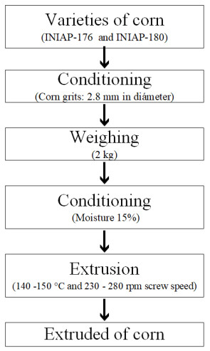
Ecuador has a significant genetic diversity of maize, which comes in different shapes, sizes and colors and plays a crucial role in food security. This research aimed to evaluate the physicochemical parameters of the extrusion process of two improved maize varieties (INIAP-176 and INIAP-180). The factors under study were two temperatures (140 ℃ and 150 ℃) and two screw speeds (230 rpm and 280 rpm). The applied extrusion conditions showed significant effects on the nutritional content, functional properties, texture attributes and sensory acceptability. The extruded products presented average values of 2.64% moisture, 0.61% ash, 8.54% protein, 0.61% ether extract, 1.55% crude fiber and 88.70 g/100 g were nitrogen-free extract (NFE) about dry weight of sample. Also, extrusion of the two maize varieties at a temperature of 150 ℃ and a screw speed of 280 rpm recorded high values of the expansion index and low levels of bulk density for functional properties. Instrumental texture analysis determined that the best attributes expressed as hardness, fracturability and adhesiveness in the expanded maize obtained from INIAP-176 at a speed of 280 rpm. The application of extrusion in these improved maize varieties allowed the production of high-quality snacks for the consumer.

| [1] |
Rouf Shah T, Prasad K, Kumar P (2016) Maize-A potential source of human nutrition and health: A review. Cogent Food Agric 2: 1166995. https://doi.org/10.1080/23311932.2016.1166995 doi: 10.1080/23311932.2016.1166995

|
| [2] |
Ranum P, Peña-Rosas JP, Garcia-Casal MN (2014) Global maize production, utilization, and consumption. Ann N Y Acad Sci 1312: 105–112. https://doi.org/10.1111/nyas.12396 doi: 10.1111/nyas.12396
|
| [3] | Velásquez J, Zambrano J, Peñaherrera D, et al. (2021) Guía para la producción sustentable de maíz en la Sierra ecuatoriana. Quito: Estación Experimental Santa Catalina. |
| [4] |
Yu BG, Chen XX, Zhou CX, et al. (2022) Nutritional composition of maize grain associated with phosphorus and zinc fertilization. J Food Compos Anal 114: 104775. https://doi.org/10.1016/j.jfca.2022.104775 doi: 10.1016/j.jfca.2022.104775
|
| [5] | Villavicencio J, Yánez C, Zambrano J (2017) Estado de la investigación y desarrollo tecnológico del maíz en Ecuador[Resumen]. In: Caviedes M, Albán M, Zambrano J, et al. (Eds.), Memorias de la XXⅡ Reunión Latinoamericana del Maíz, Quito: Universidad San Francisco de Quito/INIAP. |
| [6] | Caviedes C (1986) "INIAP-180: Nueva variedad de maíz de alto rendimiento". Ecuador: Estación Experimental Santa Catalina. |
| [7] | Moreno A (1984) Maíz "INIAP 176: variedad para grano y forraje". Ecuador: Estación Experimental Santa Catalina. |
| [8] | Kumar D, Jhariya AN (2013) Nutritional, medicinal and economical importance of corn: A mini review. Res J Pharm Sci 2319: 555X. |
| [9] | Ramos Quesnay LA (2002) Aspectos tecnológicos para la extrusión de cereales andinos. Lima: Universidad Agraria La Molina. |
| [10] | Bouvier JM, Campanella OH (2014) Extrusion processing technology: Food and non-food biomaterials. In: Bouvier JM, Campanella OH (Eds.), Extrusion Processing Technology: Food and Non-Food Biomaterials, John Wiley & Sons, India. https://doi.org/10.1002/9781118541685 |
| [11] |
Sahu C, Patel S, Tripathi AK (2022) Effect of extrusion parameters on physical and functional quality of soy protein enriched maize based extruded snack. Appl Food Res 2: 100072. https://doi.org/10.1016/j.afres.2022.100072 doi: 10.1016/j.afres.2022.100072
|
| [12] | Hegazy HS, El-Bedawey AEA, Rahma EH, et al. (2017) Effect of extrusion process on nutritional, functional properties and antioxidant activity of germinated chickpea incorporated corn extrudates. Am J Food Sci Nutr Res 4: 59–66. |
| [13] | Obradović V, Babić J, Šubarić D, et al. (2014) Improvement of nutritional and functional properties of extruded food products. J Food Nutr Res 53: 189–206. |
| [14] |
Offiah V, Kontogiorgos V, Falade KO (2019) Extrusion processing of raw food materials and by-products: A review. Crit Rev Food Sci Nutr 59: 2979–2998. https://doi.org/10.1080/10408398.2018.1480007 doi: 10.1080/10408398.2018.1480007
|
| [15] | Cuggino MI (2008) Desarrollo de alimentos precocidos por extrusión a base de maíz-leguminosa. Argentina: Universidad Nacional del Litoral. |
| [16] | Steel CJ, Leoro MGV, Schmiele M, et al. (2012) Thermoplastic extrusion in food processing. Thermoplast Elastomers 265: 411–487. |
| [17] |
Wang YY, Ryu GH (2013) Physicochemical and antioxidant properties of extruded corn grits with corn fiber by CO2 injection extrusion process. J Cereal Sci 58: 110–116. https://doi.org/10.1016/j.jcs.2013.03.013 doi: 10.1016/j.jcs.2013.03.013
|
| [18] | Vásquez C, Silva E, Taba S (1986) Análisis de estabilidad de rendimiento de variedades de maíz (Zea mays L.) harinoso y morocho en la Sierra del Ecuador. In: XⅡ Reunión de Maiceros de la Zona Andina, Ecuador: INIAP. |
| [19] | AOAC (2000) Official Methods of Analysis of the Association of Official Analytical Chemists International. 17 th Edn., Arlington, VA. |
| [20] | Ewers E (1965) Determination of starch by extraction and dispersion with hydrochloric acid. International Organization for Standardization, ISO/TC 93/WGL. |
| [21] |
Anderson RA (1969) Gelatinization of corn grits by roll-and extrusion-cooking. Cereal Sci Today 14: 4–12. https://doi.org/10.1002/star.19700220408 doi: 10.1002/star.19700220408
|
| [22] |
Mäkilä L, Laaksonen O, Ramos Diaz JM, et al. (2014) Exploiting blackcurrant juice press residue in extruded snacks. LWT-Food Sci Technol 57: 618–627. https://doi.org/10.1016/j.lwt.2014.02.005 doi: 10.1016/j.lwt.2014.02.005
|
| [23] |
Alvarez-Martinez L, Kondury KP, Harper JM (1988) A General Model for Expansion of Extruded Products. J Food Sci 53: 609–615. https://doi.org/10.1111/j.1365-2621.1988.tb07768.x doi: 10.1111/j.1365-2621.1988.tb07768.x
|
| [24] |
Neder-Suárez D, Amaya-Guerra C, Quintero-Ramos A, et al. (2016) Insoluble-bound phenolics in food. Molecules 21: 114–122. https://doi.org/10.3390/molecules21081064 doi: 10.3390/molecules21081064
|
| [25] | Watts B, Ylimaki G, Jeffery L, et al. (1992) Basic methods for food evaluation. Canadá: Centro Internacional de Investigaciones para el Desarrollo. |
| [26] | Di Rienzo J, Casanoves F, Balzarini MG, et al. (2015) InfoStat. Argentina: Grupo InfoStat, Universidad Nacional de Cordoba. |
| [27] | INEN (2013) Cereales y Leguminosas. Maíz molido, Sémola, Gritz. Requisitos. Quito: Servicio Ecuatoriano de Normalización. |
| [28] | Yánez C (2013) INIAP-180: "Nueva variedad de maíz de alto rendimiento." Ecuador: Estación Experimental Santa Catalina. |
| [29] | Yánez C (2013) INIAP-176: "Variedad para grano y forraje." Ecuador: Estación Experimental Santa Catalina. |
| [30] |
Ullah I, Ali M, Farooqi A (2010) Chemical and nutritional properties of some maize (Zea mays L.) varieties grown in NWFP, Pakistan. Pak J Nutr 9: 1113–1117. https://doi.org/10.3923/pjn.2010.1113.1117 doi: 10.3923/pjn.2010.1113.1117
|
| [31] | Altan A, Maskan M (2011) Development of extruded foods by utilizing food industry by-products. In: Advances in Food Extrusion Technology, CRC Press, Boca Raton, FL, 121–160. |
| [32] | Patil S, Brennan MA, Mason S, et al. (2017) Investigation of the combination of legumes and cereals in the development of extrudate snacks and its effect on physico-chemical properties and in vitro starch digestion. J Food Nutr Res 56: 32–41. |
| [33] |
Singh JP, Kaur A, Singh B, et al. (2019) Physicochemical evaluation of corn extrudates containing varying buckwheat flour levels prepared at various extrusion temperatures. J Food Sci Technol 56: 2205–2212. https://doi.org/10.1007/s13197-019-03703-y doi: 10.1007/s13197-019-03703-y
|
| [34] |
Manosalvas L, Villacrés E, Taimal R (2019) Efecto de la humedad de alimentación y temperatura de extrusión sobre el contenido nutricional de un snack a base de maíz, chocho y papa. Revista Bases de la Ciencia 4: 67–80. https://doi.org/10.33936/rev_bas_de_la_ciencia.v4i3.1911 doi: 10.33936/rev_bas_de_la_ciencia.v4i3.1911
|
| [35] | Ramachandra HG, Thejaswini ML (2015) Extrusion technology: A novel method of food processing. Int J Innovative Sci, Eng Technol 2: 358–369. |
| [36] |
Vega Soto C, Pérez-Bravo F, Mariotti-Celis MS (2023) Cantidad, estabilidad y digestibilidad de hidratos de carbono tras el proceso de extrusión: Impacto sobre el índice glicémico de harinas de consumo habitual en Chile. Revista chilena de nutrición, 50: 233–241. https://doi.org/10.4067/s0717-75182023000200233 doi: 10.4067/s0717-75182023000200233
|
| [37] |
Day L, Swanson BG (2013) Functionality of Protein-Fortified Extrudates. Compr Rev Food Sci Food Saf 12: 546–564. https://doi.org/10.1111/1541-4337.12023 doi: 10.1111/1541-4337.12023
|
| [38] |
Anuonye J, Onuh J, Egwim E, et al. (2010) Nutrient and antinutrient composition of extruded Acha/Soybean Blends. J Food Process Preserv 34: 680–691. https://doi.org/10.1111/j.1745-4549.2009.00425.x doi: 10.1111/j.1745-4549.2009.00425.x
|
| [39] | Moscicki L, Mitrus M, Wojtowicz A, et al. (2013) Extrusion-cooking of starch. In: Grundas A, Stępniewski S (Eds.), Advances in agrophysical research, InTech, Croatia, 319–346. https://doi.org/10.5772/52323 |
| [40] |
Offiah V, Kontogiorgos V, Falade KO (2019) Extrusion processing of raw food materials and by-products: A review. Crit Rev Food Sci Nutr 59: 2979–2998. https://doi.org/10.1080/10408398.2018.1480007 doi: 10.1080/10408398.2018.1480007
|
| [41] |
Liu L, Li S, Zhong Y, et al. (2017) Nutritional, physical and sensory properties of extruded products from high-amylose corn grits. Emir J Food Agric 29: 846–855. https://doi.org/10.9755/ejfa.2017.v29.i11.1494 doi: 10.9755/ejfa.2017.v29.i11.1494
|
| [42] |
Neder-Suárez D, Quintero-Ramos A, Meléndez-Pizarro CO, et al. (2021) Evaluation of the physicochemical properties of third-generation snacks made from blue corn, black beans, and sweet chard produced by extrusion. LWT 146: 111414. https://doi.org/10.1016/j.lwt.2021.111414 doi: 10.1016/j.lwt.2021.111414
|
| [43] |
Yağcı S, Göğüş F (2008) Response surface methodology for evaluation of physical and functional properties of extruded snack foods developed from food-by-products. J Food Eng 86: 122–132. https://doi.org/10.1016/j.jfoodeng.2007.09.018 doi: 10.1016/j.jfoodeng.2007.09.018
|
| [44] |
Contreras-Jiménez B, Morales-Sanchez E, Reyes-Vega ML, et al. (2014) Propiedades funcionales de harinas de maíz nixtamalizado obtenidas por extrusión a baja temperatura. CyTA-J Food 12: 263–270. https://doi.org/10.1080/19476337.2013.840804 doi: 10.1080/19476337.2013.840804
|
| [45] |
Pérez Ramos K, Elías Peñafiel C, Delgado Soriano V (2017) Bocadito con alto contenido proteico: un extruido a partir de quinua (Chenopodium quinoa Willd.), tarwi (Lupinus mutabilis Sweet) y camote (Ipomoea batatas L.). Sci Agropecu 8: 377–388. https://doi.org/10.17268/sci.agropecu.2017.04.09 doi: 10.17268/sci.agropecu.2017.04.09
|
| [46] |
Singh S, Gamlath S, Wakeling L (2007) Nutritional aspects of food extrusion: A review. Int J Food Sci Technol 42: 916–929. https://doi.org/10.1111/j.1365-2621.2006.01309.x doi: 10.1111/j.1365-2621.2006.01309.x
|
| [47] |
Valenzuela-Lagarda JL, Gutiérrez-Dorado R, Pacheco-Aguilar R (2017) Botanas expandidas a base de mezclas de harinas de calamar, maíz y papa: efecto de las variables del proceso sobre propiedades fisicoquímicas. CyTA-J Food 15: 118–124. https://doi.org/10.1080/19476337.2016.1219391 doi: 10.1080/19476337.2016.1219391
|
| [48] |
Kasprzak M, Rzedzicki Z, Wirkijowska A, et al. (2013) Effect of fibre–protein additions and process parameters on microstructure of corn extrudates. J Cereal Sci 58: 488–494. https://doi.org/10.1016/j.jcs.2013.09.002 doi: 10.1016/j.jcs.2013.09.002
|
| [49] |
Paula AM, Conti-Silva AC (2014) Texture profile and correlation between sensory and instrumental analyses on extruded snacks. J Food Eng 121: 9–14. https://doi.org/10.1016/j.jfoodeng.2013.08.007 doi: 10.1016/j.jfoodeng.2013.08.007
|
| [50] |
Szczesniak AS (2002) Texture is a sensory property. Food Qual Prefer 13: 215–225. https://doi.org/10.1016/S0950-3293(01)00039-8 doi: 10.1016/S0950-3293(01)00039-8
|
| [51] |
Halek GW, Paik SW, Chang KLB (1989) The Effect of Moisture Content on Mechanical Properties and Texture Profile Parameters of Corn Meal Extrudates. J Texture Stud 20: 43–56. https://doi.org/10.1111/j.1745-4603.1989.tb00419.x doi: 10.1111/j.1745-4603.1989.tb00419.x
|

Figures(2) / Tables(4)

Cinthya Calderón, María Quelal, Elena Villacrés, Luis Armando Manosalvas-Quiroz, Javier Álvarez, Nicole Villacis. Impact of extrusion on the physicochemical parameters of two varieties of corn (Zea mays)[J]. AIMS Agriculture and Food, 2023, 8(3): 873-888. doi: 10.3934/agrfood.2023046


 DownLoad: