When it comes to renewable energy, solar water heaters are among the fastest-growing technologies. Comparatively speaking, integrated collector-storage solar water heater systems cost less than other solar water heater designs. Therefore, both the construction and the operation of a combined collector-storage solar water heater are quite straightforward. The integrated storage solar collector coupled with reflectors has been experimentally investigated. The reflectors were insulated from the back side when working during the day hours and as insulated cover during the night hours. While comparing the combined collector-storage solar water heater with and without insulated reflectors, the results showed that the insulated reflectors increased the thermal efficiency by 23%. Furthermore, on the coldest day, the stored water reached a high of 82 degrees Celsius, though it was only 46 degrees Celsius that same morning.
Citation: Nassir D. Mokhlif, Muhammad Asmail Eleiwi, Tadahmun A. Yassen. Experimental evaluation of a solar water heater integrated with a corrugated absorber plate and insulated flat reflectors[J]. AIMS Energy, 2023, 11(3): 522-539. doi: 10.3934/energy.2023027
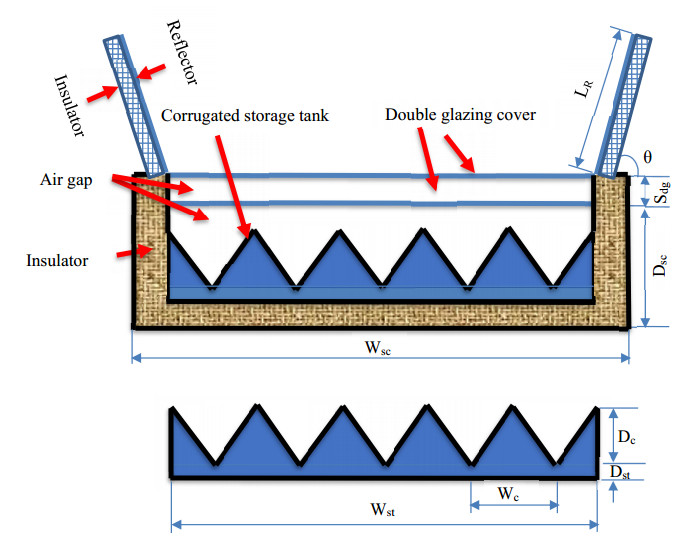
When it comes to renewable energy, solar water heaters are among the fastest-growing technologies. Comparatively speaking, integrated collector-storage solar water heater systems cost less than other solar water heater designs. Therefore, both the construction and the operation of a combined collector-storage solar water heater are quite straightforward. The integrated storage solar collector coupled with reflectors has been experimentally investigated. The reflectors were insulated from the back side when working during the day hours and as insulated cover during the night hours. While comparing the combined collector-storage solar water heater with and without insulated reflectors, the results showed that the insulated reflectors increased the thermal efficiency by 23%. Furthermore, on the coldest day, the stored water reached a high of 82 degrees Celsius, though it was only 46 degrees Celsius that same morning.

| [1] |
Oyedepo SO (2012) Energy and sustainable development in Nigeria: the way forward. Energy Sustainability Soc 2: 1–17. https://doi.org/10.1186/2192-0567-2-15 doi: 10.1186/2192-0567-2-15

|
| [2] |
Kalogirou S (1997) Design, construction, performance evaluation and economic analysis of an integrated collector storage system. Renewable Energy 12: 179–192. https://doi.org/10.1016/S0960-1481(97)00029-3 doi: 10.1016/S0960-1481(97)00029-3
|
| [3] |
Kumar R, Rosen MA (2010) Thermal performance of integrated collector storage solar water heater with corrugated absorber surface. Appl Thermal Eng 30: 1764–1768. https://doi.org/10.1016/j.applthermaleng.2010.04.007 doi: 10.1016/j.applthermaleng.2010.04.007
|
| [4] |
Mokhlif ND, Eleiwi MA, Yassen TA (2021) Experimental investigation of a double glazing integrated solar water heater with corrugated absorber surface. Mater Today Proc 42: 2742–2748. https://doi.org/10.1016/j.matpr.2020.12.714 doi: 10.1016/j.matpr.2020.12.714
|
| [5] |
Yassen TA, Mokhlif ND, Eleiwi MA (2019) Performance investigation of an integrated solar water heater with corrugated absorber surface for domestic use. Renewable Energy 138: 852–860. https://doi.org/10.1016/j.renene.2019.01.114 doi: 10.1016/j.renene.2019.01.114
|
| [6] |
Taheri Y, Ziapour BM, Alimardani K (2013) Study of an efficient compact solar water heater. Energy Convers Manage 70: 187–193. https://doi.org/10.1016/j.enconman.2013.02.014 doi: 10.1016/j.enconman.2013.02.014
|
| [7] |
Baronea PG, Buonomano A, Palmieri V, et al. (2022) A prototypal high-vacuum integrated collector storage solar water heater: Experimentation, design, and optimization through a new in-house 3D dynamic simulation model. Energy 238: 122065. https://doi.org/10.1016/j.energy.2021.122065 doi: 10.1016/j.energy.2021.122065
|
| [8] |
Bilardo M, Fraisse Pailha GM, Fabrizio E (2020) Design and experimental analysis of an Integral Collector Storage (ICS) prototype for DHW production. Appl Energy 259: 114104. https://doi.org/10.1016/j.apenergy.2019.114104. doi: 10.1016/j.apenergy.2019.114104
|
| [9] |
Harmim A, Boukar M, Amar M, et al. (2019) Simulation and experimentation of an integrated collector storage solar water heater designed for integration into building façade. Energy 166: 59–71. https://doi.org/10.1016/j.energy.2018.10.069 doi: 10.1016/j.energy.2018.10.069
|
| [10] |
Rao Anupam AS (2022) A comprehensive review on integrated collector-storage solar water heaters. Mater Today Proc 36: 15–26. https://doi.org/10.1016/j.matpr.2021.12.424 doi: 10.1016/j.matpr.2021.12.424
|
| [11] |
Sadeghi G, Mehrali M, Shahi M, et al. (2022) Experimental analysis of Shape-Stabilized PCM applied to a Direct-Absorption evacuated tube solar collector exploiting sodium acetate trihydrate and graphite. Energy Conver Manage 269: 116176. https://doi.org/10.1016/j.enconman.2022.116176 doi: 10.1016/j.enconman.2022.116176
|
| [12] | Mahmoudi A, Mehrali M, Sadeghi G, et al. (2022) Innovative direct solar receiver-storage systems for heat production. Inno-DSS Available from: https://projecten.topsectorenergie.nl/storage/app/uploads/public/623/da4/f91/623da4f91a5b5003604684.pdf. |
| [13] |
Ahmadkhani A, Sadeghi G, Safarzadeh H (2021) An in depth evaluation of matrix, external upstream and downstream recycles on a double pass flat plate solar air heater efficacy. Thermal Sci Eng Progress 21: 100789. https://doi.org/10.1016/j.tsep.2020.100789 doi: 10.1016/j.tsep.2020.100789
|
| [14] |
Mohammed MF, Eleiwi MA, Kamil KT (2020) Experimental investigation of thermal performance of improvement a solar air heater with metallic fiber. Energy Sources, Part A Recover Util Environ Eff 43: 2319–2338. https://doi.org/10.1080/15567036.2020.1833110 doi: 10.1080/15567036.2020.1833110
|
| [15] | Eleiwi MA, Mohammed MF, Kamil KT (2022) Experimental analysis of thermal performance of a solar air heater with a flat plate and metallic fiber. J Eng Sci Technol 17: 2049–2066. Available from: https://jestec.taylors.edu.my/Vol%2017%20Issue%203%20June%202022/17_3_32.pdf. |
| [16] | Talib SM, Rashid FL, Eleiwi MA (2021) The effect of air injection in a shell and tube heat exchanger. J Mech Eng Res Dev 44: 305–317. Available from: https://jmerd.net/Paper/Vol.44, No.5(2021)/305-317.pd. |
| [17] |
Eleiwi MA, Shallal HS (2020) Thermal performance of solar air heater integrated with air-water heat exchanger assigned for ambient conditions in Iraq. Int J Ambient Energy 0750: 1–22. https://doi.org/10.1080/01430750.2020.1722745 doi: 10.1080/01430750.2020.1722745
|
| [18] |
Eleiwi MA, Mokhlif ND, Saleh HF (2023) Improving the performance of the thermal energy storage of the solar water heater by using porous medium and phase change material. Energy Sour Part A: Recovery Utilization Environ Effects 45: 2013–2026. https://doi.org/10.1080/15567036.2023.2185316 doi: 10.1080/15567036.2023.2185316
|
| [19] |
Khalaf AE, Eleiwi MA, Yassen TA (2023) Enhancing the overall performance of the hybrid solar photovoltaic collector by open water cycle jet-cooling. Renewable Energy 208: 492–503. https://doi.org/10.1016/j.renene.2023.02.122 doi: 10.1016/j.renene.2023.02.122
|
| [20] |
Mohsen MS, Al-Ghandoor A, Al-Hinti I (2009) Thermal analysis of compact solar water heater under local climatic conditions. Int Commun Heat Mass Transfer 36: 962–968. https://doi.org/10.1016/j.icheatmasstransfer.2009.06.019 doi: 10.1016/j.icheatmasstransfer.2009.06.019
|
| [21] |
Sopian K, Syahri M, Abdullah S, et al. (2004) Performance of a non-metallic unglazed solar water heater with integrated storage system. Renewable Energy 29: 1421–1430. https://doi.org/10.1016/j.renene.2004.01.002 doi: 10.1016/j.renene.2004.01.002
|
| [22] | Figliola RS, Beasley D (2015) Theory and design for mechanical measurements. John Wiley Sons Available from: https://books.google.iq/books/about/Theory_and_Design_for_Mechanical_Measure.html?id = KbdYBQAAQBAJ & redir_esc = y. |
| [23] | Teussingka T, Simo-Tagne M, Njankouo JM, et al. (2023) An experimental and theoretical analysis of the dynamic response of solar drying in natural convection under rainy month of Maroua (Cameroon) of three tropical wood species. Wood Material Sci Eng 1–21. https://doi.org/10.1080/17480272.2023.2178030 |
| [24] | Wheeler AJ, Ganji AR, Krishnan VV, et al. (2010) Introduction to engineering experimentation. London, UK: Pearson, Prentice Hall, 2010. Available from: https://books.google.iq/books/about/Introduction_to_Engineering_Experimentat.html?id = crppr4QT068C & redir_esc = y. |
| [25] |
Yassen TA, Al-Kayiem HH (2016) Experimental investigation and evaluation of hybrid solar/thermal dryer combined with supplementary recovery dryer. Sol Energy 134: 284–293. https://doi.org/10.1016/j.solener.2016.05.011 doi: 10.1016/j.solener.2016.05.011
|


Figures(7) / Tables(5)

Nassir D. Mokhlif, Muhammad Asmail Eleiwi, Tadahmun A. Yassen. Experimental evaluation of a solar water heater integrated with a corrugated absorber plate and insulated flat reflectors[J]. AIMS Energy, 2023, 11(3): 522-539. doi: 10.3934/energy.2023027


 DownLoad: