Resurgence of different influenza types in China and the US in 2021

Boqiang Chen; Zhizhou Zhu; Qiong Li; Daihai He; Boqiang Chen; Zhizhou Zhu; Qiong Li; Daihai He

doi:10.3934/mbe.2023273

Mathematical Biosciences and Engineering

2023, Volume 20, Issue 4: 6327-6333. doi: 10.3934/mbe.2023273

Previous Article Next Article

Brief report Special Issues

Resurgence of different influenza types in China and the US in 2021

1.
Department of Applied Mathematics, Hong Kong Polytechnic University, Hong Kong, China
2.
BNU-HKBU United International College, Zhuhai, China

Academic Editor: Xiang-Sheng Wang

Received: 01 December 2022 Revised: 05 January 2023 Accepted: 08 January 2023 Published: 01 February 2023

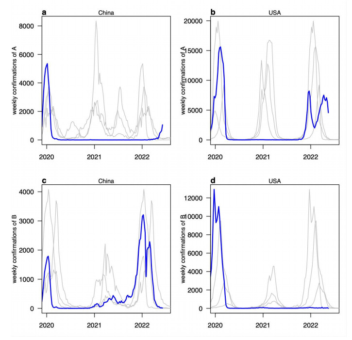
Various nonpharmaceutical interventions (NPIs) were implemented to alleviate the COVID-19 pandemic since its outbreak. The transmission dynamics of other respiratory infectious diseases, such as seasonal influenza, were also affected by these interventions. The drastic decline of seasonal influenza caused by such interventions would result in waning of population immunity and may trigger the seasonal influenza epidemic with the lift of restrictions during the post-pandemic era. We obtained weekly influenza laboratory confirmations from FluNet to analyse the resurgence patterns of seasonal influenza in China and the US. Our analysis showed that due to the impact of NPIs including travel restrictions between countries, the influenza resurgence was caused by influenza virus A in the US while by influenza virus B in China.

Keywords:

Citation: Boqiang Chen, Zhizhou Zhu, Qiong Li, Daihai He. Resurgence of different influenza types in China and the US in 2021[J]. Mathematical Biosciences and Engineering, 2023, 20(4): 6327-6333. doi: 10.3934/mbe.2023273

Related Papers:

[1]	Xianhao Zheng, Jun Wang, Kaibo Shi, Yiqian Tang, Jinde Cao . Novel stability criterion for DNNs via improved asymmetric LKF. Mathematical Modelling and Control, 2024, 4(3): 307-315. doi: 10.3934/mmc.2024025
[2]	Qin Xu, Xiao Wang, Yicheng Liu . Emergent behavior of Cucker–Smale model with time-varying topological structures and reaction-type delays. Mathematical Modelling and Control, 2022, 2(4): 200-218. doi: 10.3934/mmc.2022020
[3]	Gani Stamov, Ekaterina Gospodinova, Ivanka Stamova . Practical exponential stability with respect to $h-$ manifolds of discontinuous delayed Cohen–Grossberg neural networks with variable impulsive perturbations. Mathematical Modelling and Control, 2021, 1(1): 26-34. doi: 10.3934/mmc.2021003
[4]	Yanchao He, Yuzhen Bai . Finite-time stability and applications of positive switched linear delayed impulsive systems. Mathematical Modelling and Control, 2024, 4(2): 178-194. doi: 10.3934/mmc.2024016
[5]	M. Haripriya, A. Manivannan, S. Dhanasekar, S. Lakshmanan . Finite-time synchronization of delayed complex dynamical networks via sampled-data controller. Mathematical Modelling and Control, 2025, 5(1): 73-84. doi: 10.3934/mmc.2025006
[6]	Bangxin Jiang, Yijun Lou, Jianquan Lu . Input-to-state stability of delayed systems with bounded-delay impulses. Mathematical Modelling and Control, 2022, 2(2): 44-54. doi: 10.3934/mmc.2022006
[7]	Naveen Kumar, Km Shelly Chaudhary . Position tracking control of nonholonomic mobile robots via $H_\infty$ -based adaptive fractional-order sliding mode controller. Mathematical Modelling and Control, 2025, 5(1): 121-130. doi: 10.3934/mmc.2025009
[8]	Hongwei Zheng, Yujuan Tian . Exponential stability of time-delay systems with highly nonlinear impulses involving delays. Mathematical Modelling and Control, 2025, 5(1): 103-120. doi: 10.3934/mmc.2025008
[9]	Xipu Xu . Global existence of positive and negative solutions for IFDEs via Lyapunov-Razumikhin method. Mathematical Modelling and Control, 2021, 1(3): 157-163. doi: 10.3934/mmc.2021014
[10]	Saravanan Shanmugam, R. Vadivel, S. Sabarathinam, P. Hammachukiattikul, Nallappan Gunasekaran . Enhancing synchronization criteria for fractional-order chaotic neural networks via intermittent control: an extended dissipativity approach. Mathematical Modelling and Control, 2025, 5(1): 31-47. doi: 10.3934/mmc.2025003

Abstract

1. Introduction

Neural networks (NNs) serve as computational models that replicate the neural system of the human brain, and they are applied to address diverse problems in the field of machine learning. NNs have been widely used in various fields, including natural language processing, picture recognition, image encryption, wireline communication, finance, and business forecasting, because of its strong information processing capabilities (see ^{[1,2,3,4,5,6,7,8]}). Therefore, the stability analysis of NNs is a crucial matter, and has received a lot of attention in recent years (see ^[9,10,11]). Furthermore, the transmission of signals between neurons is subject to time-delay, which can adversely affect the performance of NNs (^[12,13]). Consequently, determining the maximum allowable delay bounds (MADBs) that can ensure the stability of NNs is an important research topic that has drawn a lot of attention ^[14]. In the existing literature, the method of delay partitioning is commonly employed for analyzing time-delay systems. In order to obtain the MADBs, on the one hand, it is necessary to require that the constructed augmented Lyapunov-Krasovskii functional (LKF) contains more delay information. On the other hand, it is necessary to relax the requirements on the matrix variables involved. The research ^[15] introduced a novel asymmetric LKF, where all matrix variables involved do not need to be symmetric or positive definite. To make the augmented LKFs contain more delay information, a novel approach to delay partitioning was presented by Guo et al. ^[16], which involves dividing the variation interval of the delay into several subintervals. A new method for determining the negativity of a quadratic function is presented in ^[17], based on its geometric information. A more thorough reciprocity convex combination inequality was used by Chen et al. ^[18] to add quadratic terms to the time derivative of a LKF. It leads to less stringent stability conditions for delayed neural network (DNNs). A novel approach to free moving points generation was introduced in ^[19] based on the work of ^[18]. Specifically, free moving points were established for synchronous movements in each subinterval. In addition, the integral inequalities can reduce conservatism by providing tighter bounds through replacement of a function with its upper or lower limit, improving our ability to predict actual results.

As previously discussed, the majority of existing research has focused on the negative condition of LKFs. However, there is a lack of investigation into its positive condition in the literature. The main work of this paper is to construct a relaxed LFK, and study the stability properties of DNNs by using a quadratic function positive definiteness method. The main contributions are summarized as follows:

(1) Distinct from prevailing methodologies, this paper presents a novel approach for demonstrating the positive definiteness of the LKF, based on the requirement that the quadratic function satisfies the positive definite condition.

(2) By employing the asymmetric LKFs methodology, we construct a relaxed LKF that incorporates delay information. The matrix variables included in this method do not require symmetry and positive definiteness.

(3) A new delay-dependent stability criterion with reduced conservatism is derived for DNNs by extending basic inequalities and incorporating the conditions of positive definiteness for the quadratic function.

Notations: $Y$ is an $n \times n$ real matrix; $Y^{T}$ is transpose of $Y$ and $Y > 0$ ; ( $Y < 0$ ) represents the positive definite (negative definite) matrix. The $*$ is a symmetric block in a symmetric matrix, $He\{Y\} = Y+Y^{T}$ . The diagonal matrix is denoted by $\operatorname{diag}\{\}$ . The n-dimensional Euclidean space is denoted by $\mathbb{R}^{n}$ and $\mathbb{R}^{n\times n}$ is the set of all $n\times n$ real matrices.

2. Preliminaries

Consider the following NNs with time-varying delay:

$\begin{equation} \begin{cases} &\dot{x}(t) = -A x(t)+B f(x(t))+C f(x(t-h_{\tau}(t))),\\ &x(t) = \rho(t), \end{cases} \end{equation}$

(2.1)

where

$x(\cdot) = col\left[x_{1}(\cdot), x_{2}(\cdot), \ldots, x_{n}(\cdot)\right]\in R^{n}$

is the neuron state vector and $\rho(t)$ is the initial condition.

$f(x(\cdot)) = col\left[f_{1}\left(x_{1}(\cdot)\right), f_{2}\left(x_{2}(\cdot)\right), \ldots, f_{n}\left(x_{n}(\cdot)\right)\right]$

denotes the activation functions.

$A = \operatorname{diag}\left\{a_{1}, a_{2}, \ldots, a_{n}\right\}$

with $a_{i} > 0$ . $B$ and $C$ are the connection matrices. The $h_{\tau}(t)$ is the time-varying delay differentiable function that satisfies $0 \leq h_{\tau}(t) \leq h$ , $\dot{h}_{\tau}(t) \leq \mu$ , where $h$ and $\mu$ are known constants. To derive our primary outcome, we need to rely on the following assumption and lemmas.

Assumption 2.1. The Lipschitz condition that the neuron activation function satisfies is as follows:

$\begin{equation*} \begin{cases} &\iota_{i}^{-} \leq \frac{f_{i}(\alpha)-f_{i}(\beta)}{\alpha-\beta}\leq\iota_{i}^{+},\\ &\alpha \neq\beta,\ f_{i}(0) = 0,\ i = 1,2,\ldots, n, \end{cases} \end{equation*}$

where $\iota_{i}^{-}$ and $\iota_{i}^{+}$ are known constants. For simplicity, denote the following matrices:

$\begin{equation*} \begin{cases} &L_{1} = \operatorname{diag} \{\iota_{1}^{-} \iota_{1}^{+}, \iota_{2}^{-} \iota_{2}^{+}, \ldots, \iota_{n}^{-} \iota_{n}^{+}\},\\ &L_{2} = \{\frac{\iota_{1}^{-}+\iota_{1}^{+}}{2}, \frac{\iota_{2}^{-}+\iota_{2}^{+}}{2}, \ldots, \frac{\iota_{n}^{-}+\iota_{n}^{+}}{2}\}. \end{cases} \end{equation*}$

Lemma 2.1. ^[20] Given any constant positive definite matrix $K \in \mathbb{R}^{n \times n}$ , for any continuous function $\chi(u)$ and $v_{1} < v_{2}$ , the following inequalities hold:

$\left(v_{2}-v_{1}\right) \int_{v_{1}}^{v_{2}} \chi^{T}(\mu) K \chi(\mu) d \mu \geq\int_{v_{1}}^{v_{2}} \chi^{\mathrm{T}}(\mu) \mathrm{d} \mu K\int_{v_{1}}^{v_{2}} \chi(\mu) \mathrm{d} \mu.$

Lemma 2.2. ^[21] Given any constant positive definite matrix $K \in \mathbb{R}^{n \times n},$ for any continuous function $\chi(u)$ and $v_{1} < v_{2}$ , the following inequalities hold:

$\begin{equation*} \begin{split} &\int_{v_{1}}^{v_{2}} \chi^{T}(\mu) K \chi(\mu) d \mu \\ &\geq \frac{1}{\left(v_{2}-v_{1}\right)}\int_{v_{1}}^{v_{2}} \chi^{\mathrm{T}}(\mu) \mathrm{d} \mu K\int_{v_{1}}^{v_{2}} \chi(\mu) \mathrm{d} \mu+\frac{3}{\left(v_{2}-v_{1}\right)}\Omega^{T}K\Omega, \end{split} \end{equation*}$

where

$\Omega = \int_{v_{1}}^{v_{2}} \chi(\mu) \mathrm{d} \mu-\frac{2}{\left(v_{2}-v_{1}\right)}\int_{v_{1}}^{v_{2}}\int_{\theta}^{v_{2}} \chi(\mu) \mathrm{d} \mu\mathrm{d} \theta.$

Lemma 2.3. ^[22] Let $R = R^{T}\in\mathbb{R}^{n \times n}$ be a positive definite matrix. If there exists matrix $X \in \mathbb{R}^{n \times n}$ such that

$\begin{bmatrix} R & X\\ \ast & R \end{bmatrix}\geq 0,$

then the following inequality holds:

$\begin{equation*} (\beta_{1}-\beta_{3})\int _{\beta _{3}}^{\beta _{1}}\dot{\chi}^{T }(\mu)R\dot{\chi}(\mu)\geq \psi ^{T }\Lambda\psi, \end{equation*}$

where

$\begin{align*} \begin{split} \psi = &col[ \chi ( \beta _{1}) ,\chi ( \beta _{2}) ,\chi ( \beta _{3})],\; \; \; \; \beta _{3} < \beta _{2} < \beta _{1},\\ \Lambda = & \begin{bmatrix} R & -R+X & -X\\ \ast & 2 R-X-X^{T } & -R+X\\ \ast & \ast & R \end{bmatrix}. \end{split} \end{align*}$

Lemma 2.4. For a quadratic function of delay,

$\xi(h_{\tau}) = ah_{\tau}^{2}(t)+b h_{\tau}(t)+c,$

where $a, b, c \in \mathbb{R}, h_{\tau} \in[0, h]$ , $\xi(h_{\tau}) > 0$ holds, if $\xi(h_{\tau})$ satisfies:

$\begin{cases} & \xi(0) > 0, \\ & \xi(h) > 0, \\ & h b+2c > 0 . \end{cases}$

Proof. We will prove Lemma 2.4 by the geometry approach.

● For $a > 0$ : $\xi(h_{\tau}(t))$ is a convex function. When $\xi(h_{\tau}(t))$ increases monotonically in $[0, \mathrm{\; h}]$ , $\xi(0) > 0$ will make $\xi(h_{\tau}(t)) > 0$ (see ); when $\xi(h_{\tau}(t))$ is monotonically decreasing in $[0, \mathrm{\; h}]$ , if $\xi(h) > 0$ , then $\xi(h_{\tau}(t)) > 0$ (see ); when $\xi(h_{\tau}(t))$ is not monotonically increasing or decreasing in $[0, h]$ , $\mathrm{D}$ is the intersection of the two tangents at $\xi(0)$ and $\xi(h)$ ; if $D > 0$ , then $\xi(h_{\tau}(t)) > 0$ (see Figure 3).

Figure 1.

$\xi(h_{\tau}(t))$ is monotonically increasing.

DownLoad: Full-Size Img PowerPoint

Figure 2.

$\xi(h_{\tau}(t))$ is monotonically decreasing.

DownLoad: Full-Size Img PowerPoint

Figure 3.

$\xi(h_{\tau}(t))$ is not monotonically increasing or decreasing.

DownLoad: Full-Size Img PowerPoint

● For $a < 0$ : $\xi(h_{\tau}(t))$ is a concave function. $\xi(h_{\tau}(t)) > 0$ in $[0, h]$ if $\xi(0) > 0$ and $\xi(h) > 0$ (see Figure 4).

Figure 4.

$\xi(h_{\tau}(t))$ is a concave function.

DownLoad: Full-Size Img PowerPoint

□

Through the above discussion, we obtained three conditions for positive definiteness of quadratic functions. In Theorem 3.1, we constructed a quadratic function form of LKFs, and under the condition of satisfying these three conditions, we can prove that LKF is positive definite.

Remark 2.1. Lemma 2.3 is a formula derived from the Bessel-Legendre integral inequality, which provides a varying estimate based on N that can help us to evaluate the upper bound of $\int _{\beta _{3}}^{\beta _{1}}\dot{\chi}^{T }(\mu)R\dot{\chi}(\mu)$ . It is apparent that Lemma 2.3 can be reduced to Lemma 2.1 when $N = 0$ (see ^[23]). In ^[17,18,19], the negative definiteness criterion of a quadratic function is utilized to demonstrate the negativity of the derivative of the LKFs. At present, there is no research that explores the use of quadratic function methods for determining the positive-definiteness property of LKFs. In this paper, the Lemma 2.4 is a condition for a quadratic function to be positive definite. In Theorem 3.1, the $h_{\tau}^{2}(t)$ term is introduced in the augmented asymmetric LKFs through the integral inequalities. On the one hand, introducing $h_{\tau}^{2}(t)$ can include more time delay information in the LKFs and reduce conservatism. On the other hand, it can make the LKFs a quadratic function.

3. Main results

The symbols used in the theorem are described here to help clarify its formulation.

$\begin{equation*} \begin{split} \eta(t) = &col [x( t) x( t-h_{\tau}( t)) x( t-h) f(x(t)) f( x( t-h_{\tau}( t)))\\ &\int _{t-h_{\tau}( t)}^{t} x( s) ds \int _{t-h}^{t} x( s) ds \int _{t-h_{\tau}( t)}^{t}\dot{x}( s)ds\int _{t-h}^{t-h_{\tau}( t)}\dot{x}( s)ds\\ &\int _{t-h_{\tau}( t)}^{t} f( x( s))ds\int _{t-h}^{t} f( x(s))ds\int _{-h}^{0}\int _{\theta }^{t} f( x( s))dsd\theta\\ &\int _{t-h}^{t}\int _{\theta }^{t} x( s) dsd\theta]\\ e_{l} = &[0_{n\times ( l-1) n}, I_{n\times n}, 0_{n\times ( 13-l) n}] \in \mathbb{R}^{n\times 13n},\\ l = &1,2,\dotsc ,13,\epsilon = \frac{1}{h}. \end{split} \end{equation*}$

Theorem 3.1. For given scalars $\mu$ and $h > 0,$ system (2.1) with time-varying delay is asymptotically stable if there exist positive definite symmetric matrices $W_{1},$ $W_{2};$ positive definite diagonal matrices $Z_{1},$ $Z_{2};$ positive definite matrices $R_{1},$ $R_{2},$ $Q_{1},$ $Q_{2};$ symmetric matrices $P_{1};$ and any appropriate dimension matrices $P_{2},$ $P_{3},$ $M,$ $N,$ $F,$ and $P = [ P_{1}, 2P_{2}, 2P_{3}]$ , such that the following linear matrix inequalities (LMIs) hold:

$\begin{equation} \xi(h_{\tau}(t),\dot{h}_{\tau}(t)) > 0, \end{equation}$

(3.1)

$\begin{equation} \begin{bmatrix} W_{2} & F\\ \ast & W_{2} \end{bmatrix}\geq 0, \quad \begin{bmatrix} \Xi _{11} & \Xi _{12}\\ \ast & \Xi _{13} \end{bmatrix} < 0, \end{equation}$

(3.2)

where

$\begin{equation*} \xi(h_{\tau}(t),\dot{h}_{\tau}(t)) = h_{\tau}^{2}(t)\Sigma_{1}+h_{\tau}(t)\Sigma_{2}+\Sigma_{3}, \end{equation*}$

$\begin{equation*} \begin{split} \Sigma_{1} = &2\epsilon^{4}e_{13}^{T}W_{1}e_{13}, \\ \Sigma_{2} = &\epsilon^{2}e_{7}^{T}R_{2}e_{7},\\ \Sigma_{3} = &e_{1}^{T}[P_{1}+W_{2}]e_{1}+\epsilon e_{6}^{T}R_{1}e_{6}\\ &+4\epsilon^{2}e_{7}^{T}W_{2}e_{7}+\epsilon e_{10}^{T}Q_{1}e_{10} +2\epsilon^{2}e_{12}^{T}Q_{2}e_{12}\\ &+12\epsilon^{4}e_{13}^{T}W_{2}e_{13}+He\{e_{1}^{T}[P_{2}-\epsilon W_{2}]e_{7}\\ &+e_{1}^{T}P_{3}e_{13}-6\epsilon^{3}e_{7}^{T}W_{2}e_{13}\},\\ \Xi _{11} = &e_{1}^{T}[2P_{2} -2P_{1} A+2hP_{3} + R_{1} +R_{2}\\ & +hW_{1} -\frac{1}{2}\epsilon W_{2}+hA^{T } W_{2} A-L_{1} Z_{1}]e_{1}\\ &+e_{2}^{T}[ \frac{1}{2}\epsilon F+\frac{1}{2}\epsilon F^{T }-( 1-\mu )R_{2} -\epsilon W_{2}\\ &-2M-2N-L_{1} Z_{2}]e_{2}-e_{3}^{T}[R_{2}+\frac{1}{2}\epsilon W_{2}]e_{3}\\ &+e_{4}^{T}[hB^{T } W_{2} B+Q_{1} +hQ_{2} -Z_{1}]e_{4}\\ &+e_{5}^{T}[h C^{T } W_{2} C -(1-\mu ) Q_{1} -Z_{2}]e_{5}\\ &+He\{e_{1}^{T}[\frac{1}{2}\epsilon W_{2} -\frac{1}{2}\epsilon F+M^{T }]e_{2}\\ &+e_{1}^{T}[\frac{1}{2}\epsilon F-P_{2}]e_{3}+e_{1}^{T}[P_{1} B- h A^{T } W_{2} B\\ &+L_{2} Z_{1}]e_{4} +e_{1}^{T}[P_{1} C -hA^{T } W_{2} C]e_{5}\\ &+e_{2}^{T}[\frac{1}{2}\epsilon W_{2} -\frac{1}{2}\epsilon F+ N]e_{3}\\ &+e_{2}^{T}[L_{2} Z_{2}]e_{5}+e_{4}^{T}[h B^{T } W_{2} C]e_{5}\},\\ \Xi _{12}& = e_{1}^{T}[-A^{T } P_{2} -P_{3}]e_{7} +e_{1}^{T}[-A^{T } P_{3}]e_{13}\\ &-e_{2}^{T}Me_{8} +e_{2}^{T}Ne_{9}+e_{4}^{T}[B^{T } P_{2}]e_{7}\\ &+e_{5}^{T}[C^{T } P_{2}]e_{7}+e_{4}^{T}[B^{T } P_{3}]e_{13}\\ &+e_{5}^{T}[C^{T } P_{3}]e_{13},\\ \Xi _{22}& = -4\epsilon e_{7}^{T} W_{1}e_{7}-\frac{1}{2}\epsilon e_{8}^{T} W_{2}e_{8}-\frac{1}{2}\epsilon e_{9}^{T} W_{2}e_{9}\\ &-\epsilon e_{11}^{T}Q_{2}e_{11}-12\epsilon^{3}e_{13}^{T}R_{2}e_{13}\\ &+He\{6\epsilon^{2} e_{7}^{T}W_{1}e_{13}\}.\\ \end{split} \end{equation*}$

Proof. Consider the following candidate LKF for system (2.1):

$\begin{equation} V( t) = \sum\limits _{i = 1}^{4} V_{i}( t), \; \; \; \; ( i = 1,2,3,4), \end{equation}$

(3.3)

where

$\begin{equation*} \begin{split} V_{1}( t) = &x^{T }( t)P\begin{bmatrix} x( t)\\ \int _{t-h}^{t} x( s) ds\\ \int _{t-h}^{t}\int _{\theta }^{t} x( s) dsd\theta \end{bmatrix},\\ V_{2}( t) = &\int _{t-h_{\tau}( t)}^{t} x^{T }( s) R_{1} x( s) ds+\int _{t-h}^{t} x^{T }( s) R_{2} x( s) ds, \end{split} \end{equation*}$

$\begin{equation*} \begin{split} V_{3}(t) = &\int _{t-h}^{t}\int _{\theta }^{t} x^{T }( s) W_{1} x( s) dsd\theta\\ &+\int _{t-h}^{t}\int _{\theta }^{t}\dot{x}^{T }( s) W_{2}\dot{x}( s) dsd\theta,\\ V_{4}( t) = &\int _{t-h_{\tau}( t)}^{t} f^{T }( x( s)) Q_{1} f( x( s)) ds\\ &+\int _{-h}^{0}\int _{t+\theta }^{t} f^{T }( x( s)) Q_{2} f( x( s)) dsd\theta. \end{split} \end{equation*}$

By Lemmas 2.1 and 2.2, we can deduce

$\begin{equation*} \begin{split} V_{2}(t) \geq&\eta^{T}(t)\{\epsilon e_{6}^{T }R_{1}e_{6}+h_{\tau} ( t)\epsilon^{2}e_{7}^{T}R_{2}e_{7}\}\eta(t),\\ V_{3}(t)\geq &\eta^{T}(t)\{2h_{\tau} ^{2}( t)\epsilon^{4}e_{12}^{T}W_{1}e_{12}+e_{1}^{T } W_{2} e_{1}\\ & -2\epsilon e_{1}^{T } W_{2} e_{7}+4\epsilon^{2} e_{7}^{T } W_{2} e_{7}\\ & -12\epsilon^{3} e_{7}^{T } W_{2} e_{13} +12\epsilon^{4} e_{13}^{T } W_{2} e_{13}\}\eta(t),\\ V_{4}(t) \geq&\eta^{T}(t)\{\epsilon e_{10}^{T } Q_{1} e_{10} +2\epsilon^{2} e_{12}^{T } Q_{2} e_{12}\}\eta(t). \end{split} \end{equation*}$

From the above derivation, we can conclude

$\begin{equation*} V(t)\geq\eta^{T}(t)[h_{\tau}^{2}(t)\Sigma_{1}+h_{\tau}(t)\Sigma_{2}+\Sigma_{3}]\eta(t). \end{equation*}$

The LKF (3.3) is positive definite if

$\xi(h_{\tau}(t),\dot{h}_{\tau}(t)) > 0.$

Next we need to derive that the derivative of LKF is negative definite. Taking the time-derivative of LKF, we have

$\begin{equation} \begin{aligned} \begin{split} \dot{V}_{1}( t) = &\eta^{T}(t)\big\{-2e_{1}^{T }[ P_{1} A-2P_{2} +2hP_{3}] e_{1} +2e_{1}^{T } P_{1} B e_{4}\\ &+2e_{4}^{T } P_{1} C e_{5} -2e_{1}^{T } A^{T } P_{2} e_{7}+2e_{4}^{T } B^{T } P_{2} e_{7}\\ &+2e_{5}^{T } C^{T } P_{2} e_{7}+2e_{1}^{T } P_{2} e_{3} -2e_{1}^{T } A^{T } P_{3} e_{13}\\ &+2e_{4}^{T } B^{T } P_{3} e_{13}+2e_{5}^{T } C^{T } P_{3} e_{13} -2e_{1}^{T } P_{3} e_{7}\big\}\eta(t),\\ \dot{V}_{2}( t) = &\eta^{T}(t)\big\{e_{1}^{T }[ R_{1} +R_{2}] e_{1} -( 1-\mu ) e_{2}^{T } R_{1} e_{2} -e_{3}^{T } R_{2}e_{3}\}\eta(t),\\ \dot{V}_{3}( t) = &-\int _{t-h}^{t} x^{T }( s) W_{1} x( s) ds+hx^{T }( t) W_{1} x( t)\\ &-\int _{t-h}^{t}\dot{x}^{T }( s) W_{2}\dot{x}( s) ds+h\dot{x}^{T }( t) W_{2}\dot{x}( t). \end{split}\end{aligned} \end{equation}$

(3.4)

Applying inequalities from Lemmas 2.1–2.3, we can obtain

$\begin{equation} \begin{aligned} \begin{split} \dot{V}_{3}(t)\leq&\eta^{T}(t)\big\{-4\epsilon e_{7}^{T } W_{1} e_{7} -12\epsilon^{3} e_{1}^{T } W_{1} e_{1}\\ & +He\left\{6\epsilon^{2} e_{7}^{T } W_{1} e_{13}\right\} -\frac{1}{2}\epsilon e_{7}^{T } W_{2} e_{7} -\frac{1}{2}\epsilon e_{8}^{T } W_{2} e_{8}\\ &+[ -Ae_{1} +Be_{4} +Ce_{5}]^{T } W_{2}[ -Ae_{1} +Be_{4} +Ce_{5}]\\ &+\gamma^{T}\Pi\gamma\}\eta(t), \end{split}\end{aligned} \end{equation}$

(3.5)

where

$\begin{equation*} \begin{split} \Pi = &-\frac{1}{2}\epsilon\begin{bmatrix} W_{2} & -W_{2} +F & -F\\ \ast & W_{2} -F-F^{T } & -W_{2} +F\\ \ast & \ast & W_{2} \end{bmatrix},\\ \gamma = &col\begin{bmatrix} e_{1} & e_{2} & e_{2} \end{bmatrix}. \end{split} \end{equation*}$

Furthermore, based on Assumption 2.1, the following condition holds for any positive definite diagonal matrices $Z_{1}$ and $Z_{2}$ :

$\begin{equation} \begin{split} 0&\leq -\sum _{j = 1}^{n} Z_{1j}\left[ f_{j}( x_{j}( t)) -\iota_{j}^{-} x_{j}( t)\right]\left[ f_{j}( x_{j}( t)) -\iota_{j}^{+} x_{j}( t)\right]\\ &\quad\ -\sum _{j = 1}^{n} Z_{2j}\left[ f_{j}( x_{j}( t-h_{\tau}( t))) -\iota_{j}^{-} x_{j}( t-h_{\tau}( t))\right]\\ &\quad\ \left[ f_{j}( x_{j}( t-h_{\tau}( t))) -\iota_{j}^{+} x_{j}( t-h_{\tau}( t))\right]. \end{split} \end{equation}$

(3.6)

For any matrices M and N, from the Newton-Leibniz integral formula, we can obtain that:

$\begin{equation*} \begin{cases} & 0 = 2x^{T}(t-h_{\tau}(t))M[x(t)-x(t-h_{\tau}(t))\\ &\quad\ \ \ -\int_{t-h_{\tau}(t)}^{t}\dot{x}(s)ds],\\ & 0 = -2x^{T}(t-h_{\tau}(t))N[x(t-h_{\tau}(t))-x(t-h)\\ &\quad\ \ \ -\int_{t-h}^{t-h_{\tau}(t)}\dot{x}(s)ds], \end{cases} \end{equation*}$

then,

$\begin{equation} \begin{cases} &0 = \eta^{T}(t)\{2e^{T }_{2}M[ e_{1} -e_{2}-e_{8}]\}\eta(t),\\ &0 = \eta^{T}(t)\{-2e^{T }_{2}N[e_{2}-e_{3} -e_{9}]\}\eta(t). \end{cases} \end{equation}$

(3.7)

By adding the (3.4)–(3.7) together, we can obtain

$\begin{equation} \dot{V}(t)\leq\eta^{T}(t)\begin{bmatrix} \Xi _{11} & \Xi _{12}\\ \ast & \Xi _{13} \end{bmatrix}\eta(t). \end{equation}$

(3.8)

Therefore, the proof has been completed. □

Remark 3.1. The purpose of constructing an augmented LKF is to extract more information from the system. By introducing new variables and parameters, the augmented LKF can describe the dynamic characteristics of the system in greater detail, helping us to better understand and analyze system behavior. Typically, in order to satisfy the stability conditions of an augmented LKF, the matrix variables involved need to be positive definite and symmetric. This is because in control theory, positive definite matrices and symmetric matrices have good properties that can ensure the nonnegativity and convexity of the LKF ^[24]. When requiring all matrix variables in the designed augmented LKFs to be positive definite and symmetric, it may lead to increased conservatism. This is because the restrictions of positive definiteness and symmetry narrow down the set of available LKFs, possibly failing to capture all system dynamics.

Remark 3.2. Inspired by ^[15], a relaxed and asymmetric LKF is constructed in this paper. The involved matrix variables do not require them to be all positive definite or symmetric in this LKF. By utilizing the condition that the quadratic function is positive definite, the proposed Lemma 2.4 ensures the positive definiteness of the LKF. Furthermore, when combined with certain extended fundamental inequalities, Theorem 1 is less conservative compared to some of the existing literature.

4. Numerical example

This section uses a numerical example to demonstrate the feasibility of the proposed approach.

Example 4.1. Consider DNNs (2.1), with the following system parameters:

$\begin{equation*} \begin{split} A& = \begin{bmatrix} 1.5&0\\ 0&1.7 \end{bmatrix},\\ L_{1} & = diag\{0, 0\},\\ L_{2} & = diag\{0.15, 0.4\},\\ B& = \begin{bmatrix} 0.0503 &0.0454\\ 0.0987& 0.2075 \end{bmatrix},\\ C& = \begin{bmatrix} 0.2381&0.9320\\ 0.0388&0.5062 \end{bmatrix}.\\ \end{split} \end{equation*}$

Solving the LMI in Theorem 3.1 yields the MADBs. shows the MADBs of Example 1 with various $\mu$ by the obtained Theorem 3.1. Compared to some recent results in other literature both theoretically and numerically. It is undeniably established that this paper's results are significantly better than some reported. Based on the data presented in , the MADBs system (2.1) yields a value of 11.8999 for $\mu$ = 0.4.

Table 1. The MADBs of

$h$ with various

$\mu$ for Example 1.

Methods	$\mu$ =0.4	$\mu$ =0.45	$\mu$ =0.5	$\mu$ =0.55
^[25] Theorem 1	7.6697	6.7287	6.4126	6.2569
^[26] Theorem 2.1 (m=6)	8.970	7.663	7.115	6.855
^[27] Theorem 1	10.2637	9.0586	9.0586	9.1910
^[28] Theorem 2	10.4371	9.1910	8.6957	8.3806
^[29] Theorem 2	10.5730	9.3566	8.8467	8.5176
Theorem 3.1	11.8999	11.4345	10.1016	9.8864
Improvement	19.472%	26.543%	20.550%	20.697%

| Show Table

DownLoad: CSV

In addition, we use different initial values ( $x_{1}(0) = col[0.5, 0.8], x_{2}(0) = col[-0.2, 0.8]$ ) and

$f(x(t)) = col\begin{bmatrix}0.3tanh(x_{1}(t)) &0.8tanh(x_{2}(t))\end{bmatrix}$

to obtain the state trajectory of the system (2.1). The graph of state trajectories show that all state trajectories ultimately converge to the equilibrium point, albeit with varying time requirements (Figures 5–8). Finally, numerical simulation results show that our proposed method is effective and the new stability criterion obtained is feasible.

Figure 5. State response of the DNNs (2.1) with

$x_{1}(0) = col[0.5, 0.8]$ ,

$\mu = 0.4$ , MADBs

$= 11.8999$ .

DownLoad: Full-Size Img PowerPoint

Figure 6. State response of the DNNs (2.1) with

$x_{1}(0) = col[0.5,0.8]$ ,

$\mu = 0.55$ , MADBs

$= 9.8864$ .

DownLoad: Full-Size Img PowerPoint

Figure 7. State response of the DNNs (2.1) with

$x_{2}(0) = col[-0.2,0.8]$ ,

$\mu = 0.4$ , MADBs

$= 11.8999$ .

DownLoad: Full-Size Img PowerPoint

Figure 8. State response of the DNNs (2.1) with

$x_{2}(0) = col[-0.2, 0.8]$ ,

$\mu = 0.55$ , MADBs

$= 9.8864$ .

DownLoad: Full-Size Img PowerPoint

5. Conclusions

The main focus of this study is on the stability analysis of NNs with time-varying delays. To improve upon existing literature, this paper has proposed a quadratic method for proving the LKF positive definite. A relaxed LKFs has been constructed based on this method, which contains more information about the time delay and allows for more relaxed requirements on the matrix variables. Using LMIs, a new stability criterion with lower conservatism has been derived. These improvements make the stability criteria applicable in a wider range of scenarios. The numerical examples illustrate the feasibility of the proposed approach.

Use of AI tools declaration

Throughout the preparation of this work, we utilized the AI-based proofreading tool "Grammarly" to identify and correct grammatical errors. Subsequently, we thoroughly examined and made any additional edits to the content as required. We take complete responsibility for the content of this publication.

Acknowledgments

This work was supported by the National Natural Science Foundation of China under Grant (No. 12061088), the Key R & D Projects of Sichuan Provincial Department of Science and Technology (2023YFG0287 and Sichuan Natural Science Youth Fund Project (No. 24NSFSC7038).

Conflict of interest

There are no conflicts of interest regarding this work.

References

[1]	N. Jones, How COVID-19 is changing the cold and flu season, Nature, 588 (2020), 388−390. https://doi.org/10.1038/d41586-020-03519-3 doi: 10.1038/d41586-020-03519-3
[2]	CDC, 2020-2021 Flu season summary [cited 2022 September 05]. Available from: https://www.cdc.gov/flu/season/faq-flu-season-2020-2021.htm.
[3]	D. He, R. Lui, L. Wang, C. K. Tse, L. Yang, L. Stone, Global spatio-temporal patterns of influenza in the post-pandemic era, Sci. Rep., 5 (2015), 1−11. https://doi.org/10.1038/srep11013 doi: 10.1038/srep11013
[4]	S. T. Ali, Y. C. Lau, S. Shan, S. Ryu, Z. Du, L. Wang, et al., Prediction of upcoming global infection burden of influenza seasons after relaxation of public health and social measures for COVID-19 pandemic, Lancet, 2022 (2022). http://dx.doi.org/10.2139/ssrn.4063811 doi: 10.2139/ssrn.4063811
[5]	A. Flahault, V. Dias-Ferrao, P. Chaberty, K. Esteves, A. J. Valleron, D. Lavanchy, FluNet as a tool for global monitoring of influenza on the Web, JAMA, 280 (1998), 1330−1332. https://doi.org/10.1001/jama.280.15.1330 doi: 10.1001/jama.280.15.1330
[6]	M. Chinazzi, J. T. Davis, M. Ajelli, C. Gioannini, M. Litvinova, S. Merler, et al., The effect of travel restrictions on the spread of the 2019 novel coronavirus (COVID-19) outbreak, Science, 368 (2020), 395−400. https://doi.org/10.1126/science.aba9757 doi: 10.1126/science.aba9757
[7]	A. Nowrasteh, A. C. Forrester, How US Travel Restrictions on China Affected the Spread of COVID-19 in the United States, JSTOR, 2020 (2020). Available from: https://www.jstor.org/stable/resrep24847?seq=2.
[8]	T. J. Christensen, A modern tragedy? COVID-19 and U.S.-China relations, Brookings Institution, 2020. Available from: https://www.brookings.edu/wp-content/uploads/2020/05/FP_20200507_covid_us_china_christensen_v2.pdf.
[9]	F. Parino, L. Zino, M. Porfiri, A. Rizzo, Modelling and predicting the effect of social distancing and travel restrictions on COVID-19 spreading, J. R. Soc. Interface, 18 (2021), 20200875. https://doi.org/10.1098/rsif.2020.0875 doi: 10.1098/rsif.2020.0875
[10]	K. Linka, M. Peirlinck, F. S. Costabal, E. Kuhl, Outbreak dynamics of COVID-19 in Europe and the effect of travel restrictions, Comput. Methods Biomech. Biomed. Eng., 23 (2020), 710−717. https://doi.org/10.1080/10255842.2020.1759560 doi: 10.1080/10255842.2020.1759560
[11]	L. Zheng, J. Qi, J. Wu, M. Zheng, Changes in influenza activity and circulating subtypes during the COVID-19 outbreak in China, Front. Med., 2022 (2022), 627. https://doi.org/10.3389/fmed.2022.829799 doi: 10.3389/fmed.2022.829799
[12]	S. Han, T. Zhang, Y. Lyu, S. Cai, P. Dai, J. Zheng, et al., The incoming influenza season—China, the United Kingdom, and the United States, 2021–2022, China CDC Wkly., 3 (2021), 1039−1045. https://doi.org/10.46234/ccdcw2021.253 doi: 10.46234/ccdcw2021.253
[13]	B. J. Cowling, S. T. Ali, T. W. Y. Ng, T. K. Tsang, J. C. M. Li, M. W. Fong, et al., Impact assessment of non-pharmaceutical interventions against coronavirus disease 2019 and influenza in Hong Kong: an observational study, Lancet Public Health, 5 (2020), e279−e288. https://doi.org/10.1016/S2468-2667(20)30090-6 doi: 10.1016/S2468-2667(20)30090-6
[14]	A. Merced-Morales, P. Daly, A. I. A. Elal, N. Ajayi, E. Annan, A. Budd, et al., Influenza activity and composition of the 2022–23 influenza vaccine—United States, 2021–22 season, Morb. Mortal. Wkly. Rep., 71 (2022), 913. https://doi.org/10.15585/mmwr.mm7129a1 doi: 10.15585/mmwr.mm7129a1
[15]	M. Koutsakos, A. K. Wheatley, K. Laurie, S. J. Kent, S. Rockman, Influenza lineage extinction during the COVID-19 pandemic? Nat. Rev. Microbiol., 19 (2021), 741−742. https://doi.org/10.1038/s41579-021-00642-4 doi: 10.1038/s41579-021-00642-4
[16]	CDC, Influenza vaccination coverage for persons 6 months and older [cited 2023 January 05]. Available from: https://www.cdc.gov/flu/fluvaxview/interactive-general-population.htm.
[17]	J. Yang, K. E. Atkins, L. Feng, M. Pang, Y. Zheng, X. Liu, et al., Seasonal influenza vaccination in China: landscape of diverse regional reimbursement policy, and budget impact analysis, Vaccine, 34 (2016), 5724−5735. https://doi.org/10.1016/j.vaccine.2016.10.013 doi: 10.1016/j.vaccine.2016.10.013
[18]	J. Fan, S. Cong, N. Wang, H. Bao, B. Wang, Y. Feng, et al., Influenza vaccination rate and its association with chronic diseases in China: results of a national cross-sectional study, Vaccine, 38 (2020), 2503−2511. https://doi.org/10.1016/j.vaccine.2020.01.093 doi: 10.1016/j.vaccine.2020.01.093

mbe-20-04-273-supplementary.pdf

This article has been cited by:

Luyao Li, Licheng Fang, Huan Liang, Tengda Wei, Observer-based event-triggered impulsive control of delayed reaction-diffusion neural networks, 2025, 22, 1551-0018, 1634, 10.3934/mbe.2025060

Reader Comments

Your name:*

Email:*
© 2023 the Author(s), licensee AIMS Press. This is an open access article distributed under the terms of the Creative Commons Attribution License (http://creativecommons.org/licenses/by/4.0)

通讯作者: 陈斌, bchen63@163.com

1.
沈阳化工大学材料科学与工程学院沈阳 110142

Mathematical Biosciences and Engineering

4.4

Metrics

Article views(2620) PDF downloads(139) Cited by(9)

Preview PDF

Download XML

Export Citation

Article outline

Show full outline

Figures and Tables

Figures(2)

Mathematical Biosciences and Engineering

Resurgence of different influenza types in China and the US in 2021

Related Papers:

Abstract

1. Introduction

2. Preliminaries

3. Main results

4. Numerical example

5. Conclusions

Use of AI tools declaration

Acknowledgments

Conflict of interest

References

This article has been cited by:

Reader Comments

通讯作者: 陈斌, bchen63@163.com

Metrics

Figures and Tables

Other Articles By Authors

Catalog

Mathematical Biosciences and Engineering

Resurgence of different influenza types in China and the US in 2021

Related Papers:

Abstract

1. Introduction

2. Preliminaries

3. Main results

4. Numerical example

5. Conclusions

Use of AI tools declaration

Acknowledgments

Conflict of interest

References

This article has been cited by:

Reader Comments

通讯作者: 陈斌, bchen63@163.com

Metrics

Figures and Tables

Other Articles By Authors

Related pages

Tools

Export File

Citation

Format

Content

Catalog