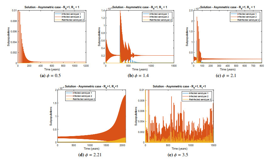
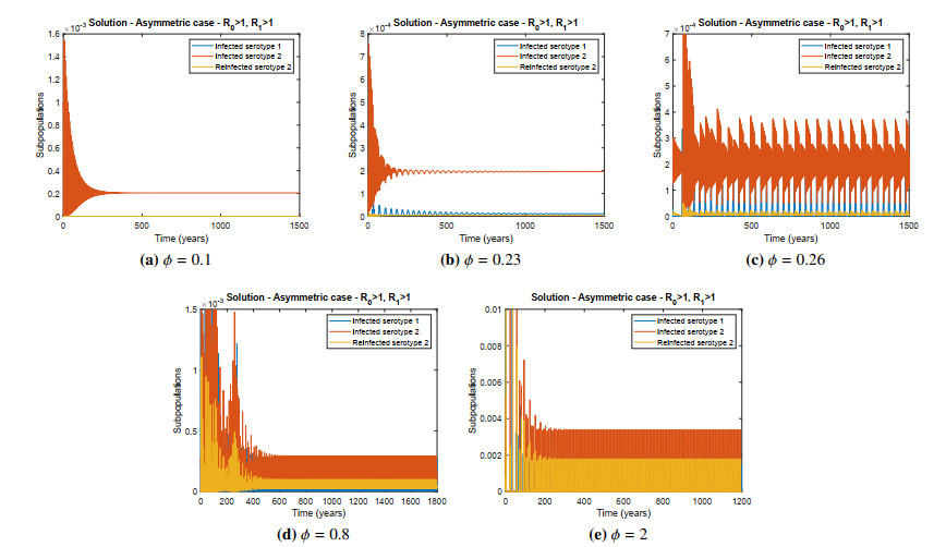
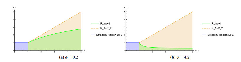
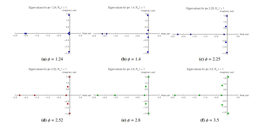
Dengue fever is endemic in tropical and subtropical countries, and certain important features of the spread of dengue fever continue to pose challenges for mathematical modelling. Here we propose a system of integro-differential equations (IDE) to study the disease transmission dynamics that involve multi-serotypes and cross immunity. Our main objective is to incorporate and analyze the effect of a general time delay term describing acquired cross immunity protection and the effect of antibody-dependent enhancement (ADE), both characteristics of Dengue fever. We perform qualitative analysis of the model and obtain results to show the stability of the epidemiologically important steady solutions that are completely determined by the basic reproduction number and the invasion reproduction number. We establish the global dynamics by constructing a suitable Lyapunov functional. We also conduct some numerical experiments to illustrate bifurcation structures, indicating the occurrence of periodic oscillations for a specific range of values of a key parameter representing ADE.
Citation: Vanessa Steindorf, Sergio Oliva, Jianhong Wu. Cross immunity protection and antibody-dependent enhancement in a distributed delay dynamic model[J]. Mathematical Biosciences and Engineering, 2022, 19(3): 2950-2984. doi: 10.3934/mbe.2022136
Dengue fever is endemic in tropical and subtropical countries, and certain important features of the spread of dengue fever continue to pose challenges for mathematical modelling. Here we propose a system of integro-differential equations (IDE) to study the disease transmission dynamics that involve multi-serotypes and cross immunity. Our main objective is to incorporate and analyze the effect of a general time delay term describing acquired cross immunity protection and the effect of antibody-dependent enhancement (ADE), both characteristics of Dengue fever. We perform qualitative analysis of the model and obtain results to show the stability of the epidemiologically important steady solutions that are completely determined by the basic reproduction number and the invasion reproduction number. We establish the global dynamics by constructing a suitable Lyapunov functional. We also conduct some numerical experiments to illustrate bifurcation structures, indicating the occurrence of periodic oscillations for a specific range of values of a key parameter representing ADE.

| [1] | World Health Organization (WHO), 2018. Available from: https://www.who.int/news-room/fact-sheets/detail/dengue-and-severe-dengue. |
| [2] | D. J. Gubler, E. E. Ooi, S. Vasudevan, J. Farrar, Dengue and dengue hemorrhagic fever, CABI (2014). |
| [3] |
M. G. Guzman, M. Alvarez, S. B. Halstead, Secondary infection as a risk factor for dengue hemorrhagic fever/dengue shock syndrome: an historical perspective and role of antibody-dependent enhancement of infection, {Arch. Virol.}, 158 (2013), 1445–1459. https://doi.org/10.1007/s00705-013-1645-3. doi: 10.1007/s00705-013-1645-3

|
| [4] |
N. G. Reich, S. Shrestha, A. A. King, P. Rohani, J. Lessler, S. Kalayanarooj, et al., Interactions between serotypes of dengue highlight epidemiological impact of cross-immunity, {J. R. Soc. Interface}, 10 (2013), 4–14. https://doi.org/10.1098/rsif.2013.0414. doi: 10.1098/rsif.2013.0414
|
| [5] |
B. Adams, M. Boots, Modelling the relationship between antibody-dependent enhancement and immunological distance with application to dengue, {J. Theor. Biol.}, 242 (2006), 337–346. https://doi.org/10.1016/j.jtbi.2006.03.002. doi: 10.1016/j.jtbi.2006.03.002
|
| [6] |
S. Bianco, L. B. Shaw, I. B. Schwartz, Epidemics with multistrain interactions: the interplay between cross immunity and antibody-dependent enhancement, {Chaos}, 19 (2009), 043123. https://doi.org/10.1063/1.3270261. doi: 10.1063/1.3270261
|
| [7] |
L. Billings, I. B. Schwartz, L. B. Shaw, M. McCrary, D. S. Burke, D. A. T. Cummings, Instabilities in multiserotype disease models with antibody-dependent enhancement, {J. Theor. Biol.}, 246 (2007), 18–27. https://doi.org/10.1016/j.jtbi.2006.12.023. doi: 10.1016/j.jtbi.2006.12.023
|
| [8] |
K. Hu, C. Thoens, S. Bianco, S. Edlund, M. Davis, J. Douglas, et al., The effect of antibody-dependent enhancement, cross immunity, and vector population on the dynamics of dengue fever, { J. Theor. Biol.}, 319 (2013), 62–74. https://doi.org/10.1016/j.jtbi.2012.11.021. doi: 10.1016/j.jtbi.2012.11.021
|
| [9] | M. Aguiar, N. Stollenwerk, A new chaotic attractor in a basic multi-strain epidemiological model with temporary cross-immunity, preprint (2007), arXiv: 0704.3174v1. |
| [10] |
M. Aguiar, B. Kooi, N. Stollenwerk, Epidemiology of dengue fever: A model with temporary cross immunity and possibly secondary infection shows bifurcations and chaotic behaviors in wide parameter region, Math. Model. Nat. Phenom., 3 (2008), 48–70. https://doi.org/10.1051/mmnp:2008070. doi: 10.1051/mmnp:2008070
|
| [11] |
B. W. Kooi, M. Aguiar, N. Stollenwerk, Analysis of an asymmetric two-strain dengue model, Math. Biosci., 248 (2014), 128–139. https://doi.org/10.1016/j.mbs.2013.12.009. doi: 10.1016/j.mbs.2013.12.009
|
| [12] | P. Van den Driessche, Some epidemiological Models with delays. In: Differential Equations and Application to biology and to Industry, World Sci. (1996), 507–520. |
| [13] |
K. Nah, Y. Nakata, G. Rost, Malaria dynamics with long incubation period in host, Comp. Math. with App., 68 (2014), 915–930. https://doi.org/10.1016/j.camwa.2014.05.001. doi: 10.1016/j.camwa.2014.05.001
|
| [14] |
D. Chen, Z. Xu, Global dynamics of a delayed diffusive two-strain disease model, Diff. Eq. App., 8 (2016), 99–122. https://doi.org/10.7153/dea-08-07. doi: 10.7153/dea-08-07
|
| [15] | J. Guan, L. Wu., M. Chen, X. Dong, H. Tang, Z. Chen, The stability and Hopf Bifurcation of the dengue fever model with time delay, It. J. Pure App. Math., 37 (1973), 139–156. |
| [16] |
K. Hattaf, A. A. Lashari, Y. Louartassi, N. Yousfi, A delayed SIR epidemic model with a general incidence rate, Elect. J. Qual. The. Differ. Equ., 3 (2013), 1–9. https://doi.org/10.14232/ejqtde.2013.1.3. doi: 10.14232/ejqtde.2013.1.3
|
| [17] |
C. Huang, J. Cao, F. Wen, X. Yang, X., Stability Analysis of SIR Model with Distributed Delay on Complex Networks, PLoS ONE, 11 (2016), e0158813. https://doi.org/10.1371/journal.pone.0158813. doi: 10.1371/journal.pone.0158813
|
| [18] |
J. Xu, Y. Geng, Y. Zhou, Global stability of a multi-group model with distributed delay and vaccination, Math. Meth. App. Sci., 40 (2017), 1475–1486. https://doi.org/10.1002/mma.4068. doi: 10.1002/mma.4068
|
| [19] |
L. C. Katzelnick, L. Gresh, M. E. Halloran, J. C. Mercado, G. Kuan, A. Gordon, et al., Antibody-dependent enhancement of severe dengue disease in humans, { Science}, 358 (2017), 929–932. https://doi.org/10.1126/science.aan6836. doi: 10.1126/science.aan6836
|
| [20] |
A. Rothman, Immunity to dengue virus: a tale of original antigenic sin and tropical cytokine storms, Nat. Rev. Immunol., 11 (2011), 532–543. https://doi.org/10.1038/nri3014. doi: 10.1038/nri3014
|
| [21] | L. Wang, Y. Li, L. Pang, Dynamics Analysis of an Epidemiological Model with media impact and two delays, Math. Prob. Eng., (2016), Article ID 1598932. https://doi.org/10.1155/2016/1598932. |
| [22] | K. L. Cooke, P. Van den Driessche, Analysis of an SEIRS epidemic model with two delays, J. Math. Biol., 35 (1996), 240–260. |
| [23] |
P. Van den Driessche, L. Wang, X. Zou, Modeling diseases with latency and relapse, Math. Biosci. Eng., 4 (2007), 205–219. https://doi.org/10.3934/mbe.2007.4.205. doi: 10.3934/mbe.2007.4.205
|
| [24] | P. Van den Driessche, J. Watmough, Further Notes on the Basic Reproduction Number, Math. Ep., (2008), 159–178. |
| [25] | M. Martcheva, Introduction to Mathematical Epidemiology, Springer, New York (2015). |
| [26] |
C. S. VinodKumar, N. K. Kalapannavar, K. G. Basavarajappa, D. Sanjay, C. Gowli, N. G. Nadig, et al., Episode of coexisting infections with multiple dengue virus serotypes in central Karnataka, J. Inf. Public. Health, 6 (2013), 302–306. https://doi.org/10.1016/j.jiph.2013.01.004. doi: 10.1016/j.jiph.2013.01.004
|
| [27] | F. Brauer, Asymptotic stability of a class of integro-differential equation, J. Diff. Eq., 28 (1978), 180–188. |
| [28] | R. K. Miller, Nonlinear Volterra Integral Equations, W. A. Benjamin, California, (1971). |
| [29] | H. K. Hethcote, H. W. Stech, P. Van den Driessche, Nonlinear Oscillations in Epidemic Models, J. Appl. Math., 40 (1981). |
| [30] | R. K. Miller, Asymptotic stability properties of linear Volterra Integro-differential equations, J. Diff. Eq., 10 (1971), 485–506. |
| [31] |
X. Feng, K. Wang, F. Zhang, Z. Teng, Threshold dynamics of a nonlinear multigroup epidemic model with two infinite distributed delays, Math. Meth. Appl. Sci., 40 (2016), 2762–2771. https://doi.org/10.1002/mma.4196. doi: 10.1002/mma.4196
|
| [32] |
J. Wang, Y. Takeuchi, A multi-group SVEIR epidemic model with distributed delay and vaccination, Int. J. Bio., 5 (2012), 1260001. https://doi.org/10.1142/S1793524512600017. doi: 10.1142/S1793524512600017
|
| [33] |
M. Y. Li, Z. Shuai, C. Wang, Global stability of multi-group epidemic models with distributed delay, J. Math. Anal. Appl., 361 (2010), 38–47. https://doi.org/10.1016/j.nonrwa.2011.11.016. doi: 10.1016/j.nonrwa.2011.11.016
|
| [34] |
G. Röst, J. Wu, SEIR epidemiological model with varying infectivity and infinite delay, Math. Bio. Eng, 5 (2008), 389–402. https://doi.org/10.3934/mbe.2008.5.389. doi: 10.3934/mbe.2008.5.389
|
| [35] | S. I. Grossman, R. K. Miller, Nonlinear Volterra Integro-differential systems with $L^1$-Kernels, J. Diff. Eq., 13 (1973), 551–556. |
| [36] | T. A. Burton, Volterra Integral and Differential Equations, in Mathematics in Science and Engineerin, Elsevier, (2005), 1–355. |
| [37] | J. P. LaSalle, The Stability of Dynamical Systems, In Regional Conference Series in Applied Mathematics, SIAM, USA (1976). |
| [38] | IBGE/DPE/Coordenação de População e Indicadores Sociais, Gerência de Estudos e Análises da Dinâmica Demográfica, 2018. Avaiable from: http://tabnet.datasus.gov.br/cgi/idb2012/a11tb.htm. |
| [39] | World Health Organization (2009) Dengue: Guidelines for Diagnosis, Treatment, Prevention and Control, New edition, A joint publication of the World Health Organization (WHO) and the Special Programme for Research and Training in Tropical Diseases (TDR), 2009. Available from: https://www.who.int/tdr/publications/documents/dengue-diagnosis.pdf. |
| [40] | N. Ferguson, R. Anderson, S. Gupta, The effect of antibody-dependent enhancement on the transmission dynamics and persistence of multiple strain pathogens, Proc. Natl. Acad. Sci., 96 (1999), 790–794. |
| [41] |
S. B. Maier, X. Huanga, E. Massad, M. Amaku, M. N. Burattini, D. Greenhalgh, Analysis of the optimal vaccination age for dengue in Brazil with a tetravalent dengue vaccine, Math. Biosci., 294 (2017), 15—32. https://doi.org/10.1016/j.mbs.2017.09.004. doi: 10.1016/j.mbs.2017.09.004
|
| [42] |
E. Massad, F. A. Coutinho, M. N. Burattini, L. F. Lopez, The risk of yellow fever in a dengue-infested area, {Trans. R. Soc. Trop. Med. Hyg.}, 95 (2001), 370–374. https://doi.org/10.1016/s0035-9203(01)90184-1. doi: 10.1016/s0035-9203(01)90184-1
|
| [43] |
R. C. Reiner, S. T. Stoddard, B. M. Forshey, A. A. King, A. M. Ellis, A. L. Lloyd, et al., Time-varying, serotype-specific force of infection of dengue virus, Proc. Natl. Acad. Sci., 111 (2014), E2694–E2702. https://doi.org/10.1073/pnas.1314933111. doi: 10.1073/pnas.1314933111
|
| [44] | N. M. Ferguson, C. A. Donnelly, R. M. Anderson, Transmission dynamics and epidemiology of dengue: Insights from age-stratified sero-prevalence surveys, { Phil. Trans. R. Soc. B Biol. Sci.}, 354 (1999), 757—768. |
| [45] | L. Edelstein-Keshet, Mathematical Models in Biology, SIAM PA, USA (2005). |
| [46] | J. D. Murray, Mathematical Biology I. An Introduction, 3rd ed, Springer (2002). |
| [47] | S. Lynch, Dynamical systems with applications using MATLAB, Springer, (2004). |
| [48] |
G. Huang, A. Liu, A note on global stability for a heroin epidemic model with distributed delay, App. Math. Let., 26 (2013), 687–691. https://doi.org/10.1016/j.aml.2013.01.010. doi: 10.1016/j.aml.2013.01.010
|
| [49] | J. Hale, S. M. V. Lunel, Introduction to Functional Differential Equations, Vol. 9, Applied Mathematical Science, New York, (1993). |
Figures(12) / Tables(2)

Vanessa Steindorf, Sergio Oliva, Jianhong Wu. Cross immunity protection and antibody-dependent enhancement in a distributed delay dynamic model[J]. Mathematical Biosciences and Engineering, 2022, 19(3): 2950-2984. doi: 10.3934/mbe.2022136


 DownLoad: