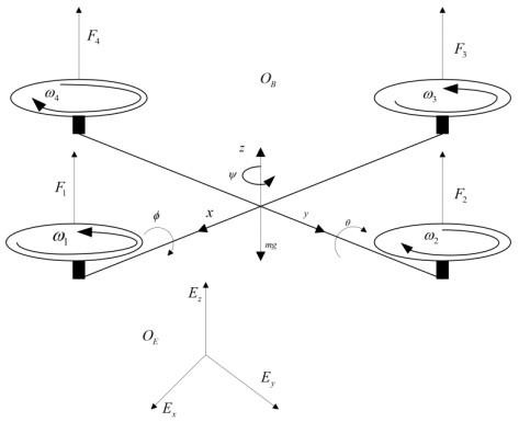
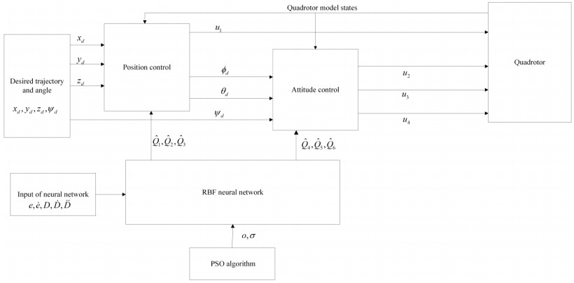
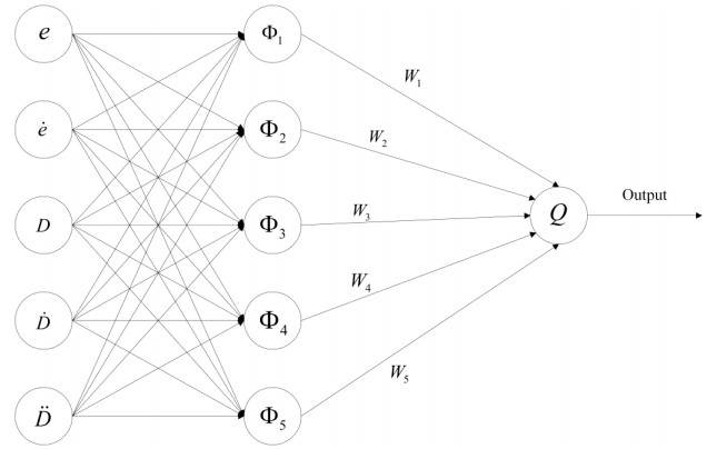
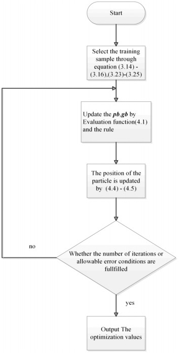
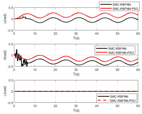
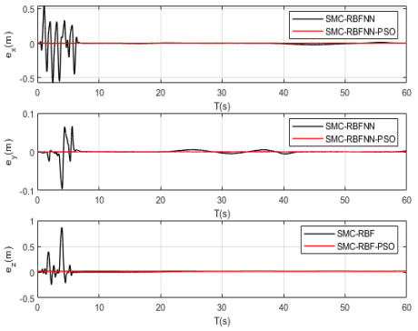
In this paper, optimized radial basis function neural networks (RBFNNs) are employed to construct a sliding mode control (SMC) strategy for quadrotors with unknown disturbances. At first, the dynamics model of the controlled quadrotor is built, where some unknown external disturbances are considered explicitly. Then SMC is carried out for the position and the attitude control of the quadrotor. However, there are unknown disturbances in the obtained controllers, so RBFNNs are employed to approximate the unknown parts of the controllers. Furtherly, Particle Swarm optimization algorithm (PSO) based on minimizing the absolute approximation errors is used to improve the performance of the controllers. Besides, the convergence of the state tracking errors of the quadrotor is proved. In order to exposit the superiority of the proposed control strategy, some comparisons are made between the RBFNN based SMC with and without PSO. The results show that the strategy with PSO achieves quicker and smoother trajectory tracking, which verifies the effectiveness of the proposed control strategy.
Citation: Ping Li, Zhe Lin, Hong Shen, Zhaoqi Zhang, Xiaohua Mei. Optimized neural network based sliding mode control for quadrotors with disturbances[J]. Mathematical Biosciences and Engineering, 2021, 18(2): 1774-1793. doi: 10.3934/mbe.2021092
In this paper, optimized radial basis function neural networks (RBFNNs) are employed to construct a sliding mode control (SMC) strategy for quadrotors with unknown disturbances. At first, the dynamics model of the controlled quadrotor is built, where some unknown external disturbances are considered explicitly. Then SMC is carried out for the position and the attitude control of the quadrotor. However, there are unknown disturbances in the obtained controllers, so RBFNNs are employed to approximate the unknown parts of the controllers. Furtherly, Particle Swarm optimization algorithm (PSO) based on minimizing the absolute approximation errors is used to improve the performance of the controllers. Besides, the convergence of the state tracking errors of the quadrotor is proved. In order to exposit the superiority of the proposed control strategy, some comparisons are made between the RBFNN based SMC with and without PSO. The results show that the strategy with PSO achieves quicker and smoother trajectory tracking, which verifies the effectiveness of the proposed control strategy.

| [1] |
N. Fethalla, M. Saad, H. Michalska, J. Ghommam, Robust observer-based dynamic sliding mode controller for a quadrotor UAV, IEEE Access, 6 (2018), 45846–45859. doi: 10.1109/ACCESS.2018.2866208

|
| [2] | A. Levant, Principles of 2-sliding mode design, Automatica, 43 (2007), 576–586. |
| [3] | R. Xu, Ü. Özgüner, Sliding mode control of a class of underactuated systems, Automatica, 44 (2008), 233–241. |
| [4] |
D. Lee, H. J. Kim and S. Sastry, Feedback linearization vs. adaptive sliding mode control for a quadrotor helicopter, Int. J. Control Autom. Syst., 7(2009), 419–428. doi: 10.1007/s12555-009-0311-8
|
| [5] |
E. H. Zheng, J. J. Xiong, J. L. Luo, Second order sliding mode control for a quadrotor UAV, ISA Trans., 53 (2014), 1350–1356. doi: 10.1016/j.isatra.2014.03.010
|
| [6] |
J. J. Xiong, E. H. Zheng, Position and attitude tracking control for a quadrotor UAV, ISA Trans., 53 (2014), 725–731. doi: 10.1016/j.isatra.2014.01.004
|
| [7] |
J. J. Xiong, G. B. Zhang, Global fast dynamic terminal sliding mode control for a quadrotor UAV, ISA Trans., 66 (2017), 233–240. doi: 10.1016/j.isatra.2016.09.019
|
| [8] |
H. Ríos, R. Falcón, O. A. González, A. Dzul, Continuous sliding-mode control strategies for quadrotor robust tracking: real-time application, IEEE Trans. Ind. Electron., 66 (2019), 1264–1272. doi: 10.1109/TIE.2018.2831191
|
| [9] |
B. X. Mu, K. W. Zhang and Y. Shi, Integral sliding mode flight controller design for a quadrotor and the application in a heterogeneous multi agent system, IEEE Trans. Ind. Electron., 64 (2017), 9389–9398. doi: 10.1109/TIE.2017.2711575
|
| [10] |
H. P. Wang, X. F. Ye, Y. Tian, G. Zheng, N. Christov, Model-free based terminal SMC of quadrotor attitude and position, IEEE Trans. Aerosp. Electron. Syst., 52 (2016), 2519–2528. doi: 10.1109/TAES.2016.150303
|
| [11] |
O. Mofid, S. Mobayen, Adaptive sliding mode control for finite time stability of quadrotor UAVs with parametric uncertainties, ISA Trans., 72 (2018), 1–14. doi: 10.1016/j.isatra.2017.11.010
|
| [12] |
L. Derafa, A. Benallegue, L. Fridman, Super twisting control algorithm for the attitude tracking of a four rotors UAV, J. Franklin Inst., 349 (2012), 685–699. doi: 10.1016/j.jfranklin.2011.10.011
|
| [13] |
M. Boukattaya, N. Mezghani, T. Damak, Adaptive nonsingular fast terminal sliding-mode control for the tracking problem of uncertain dynamical systems, ISA Trans., 77 (2018), 1–19. doi: 10.1016/j.isatra.2018.04.007
|
| [14] |
M. Labbadi, M. Cherkaoui, Robust adaptive nonsingular fast terminal sliding-mode tracking control for an uncertain quadrotor UAV subjected to disturbances, ISA Trans., 99 (2020), 290–304. doi: 10.1016/j.isatra.2019.10.012
|
| [15] |
B. Wang, X. Yu, L. X. Mu, Y. M. Zhang, Disturbance observer-based adaptive fault-tolerant control for a quadrotor helicopter subject to parametric uncertainties and external disturbances, Mech. Syst. Signal Proc., 120 (2019), 727–743. doi: 10.1016/j.ymssp.2018.11.001
|
| [16] | G. Q. Zhu, S. Wang, L. F. Sun, W. C. Ge, X. Y. Zhang, Output feedback adaptive dynamic surface sliding-mode control for quadrotor UAVs with tracking error constraints, Complexity, 2020 (2020), 1–23. |
| [17] | M. Labbadi, M. Cherkaoui, Robust adaptive backstepping fast terminal sliding mode controller for uncertain quadrotor UAV, Aerosp. Sci. Technol., 93 (2019), 105306. |
| [18] |
H. Razmi, S. Afshinfar, Neural network-based adaptive sliding mode control design for position and attitude control of a quadrotor UAV, Aerosp. Sci. Technol., 91 (2019), 12–27. doi: 10.1016/j.ast.2019.04.055
|
| [19] |
Y. M. Chen, Y. L. He, M. F. Zhou, Decentralized PID neural network control for a quadrotor helicopter subjected to wind disturbance, J. Cent. South Univ., 22 (2015), 168–179. doi: 10.1007/s11771-015-2507-9
|
| [20] |
S. S. Li, Y. N. Wang, J. H. Tan, Y. Zheng, Adaptive RBFNNs/integral sliding mode control for a quadrotor aircraft, Neurocomputing., 216 (2016), 126–134. doi: 10.1016/j.neucom.2016.07.033
|
| [21] |
O. Doukhi, D. J. Lee, Neural network-based robust adaptive certainty equivalent controller for quadrotor UAV with unknown disturbances, Int. J. Control Autom. Syst., 17 (2019), 2365–2374. doi: 10.1007/s12555-018-0720-7
|
| [22] |
Q. Z. Xu, Z. S. Wang, Z. Y. Zhen, Adaptive neural network finite time control for quadrotor UAV with unknown input saturation, Nonlinear Dyn., 98 (2019), 1973–1998. doi: 10.1007/s11071-019-05301-1
|
| [23] |
C. X. Mu, Y. Zhang, Learning-based robust tracking control of quadrotor with time-varying and coupling uncertainties, IEEE Trans. Neural Netw. Learn. Syst., 31 (2020), 259–273. doi: 10.1109/TNNLS.2019.2900510
|
| [24] |
Z. Li, X. Ma, Y. B. Li, Robust tracking control strategy for a quadrotor using RPD-SMC and RISE, Neurocomputing., 331 (2019), 312–322. doi: 10.1016/j.neucom.2018.11.070
|
| [25] | Y. Wang, Y. Chenxie, J. Tan, C. Wang, Y. Wang and Y. Zhang, Fuzzy radial basis function neural network PID control system for a quadrotor UAV based on particle swarm optimization, IEEE Int. Conf. Inf. Autom., (2015), 2580–2585. |
| [26] |
R. Zhang, J. Tao, R. Lu, Q. Jin, Decoupled ARX and RBF neural network modeling using PCA and GA optimization for nonlinear distributed parameter systems, IEEE Trans. Neural Netw. Learn. Syst., 29 (2018), 457–469. doi: 10.1109/TNNLS.2016.2631481
|
| [27] |
S. Q. Wang, M. Roger, J. Sarrazin, C. Lelandais-Perrault, Hyperparameter optimization of two-hidden-layer neural networks for power amplifiers behavioral modeling using genetic algorithms, IEEE Microw. Wirel. Compon. Lett., 29 (2019), 802–805. doi: 10.1109/LMWC.2019.2950801
|
| [28] |
W. J. Cai, J. H. She, M. Wu, Y. Ohyama, Disturbance suppression for quadrotor UAV using sliding-mode-observer-based equivalent-input-disturbance approach, ISA Trans., 92 (2019), 286–297. doi: 10.1016/j.isatra.2019.02.028
|
| [29] | W. K. Alqaisi, B. Brahmi, J. Ghommam, M. Saad, V. Nerguizian, Adaptive sliding mode control based on RBF neural network approximation for quadrotor, IEEE Int. Symp. Robot. Sensors Environ., (2019), 1–7. |
| [30] | J. K. Liu, X. H. Wang, Advanced sliding mode control for mechanical systems: Design, analysis and MATLAB simulation, Tsinghua University Press, Beijing, 2011. |
Figures(10) / Tables(4)

Ping Li, Zhe Lin, Hong Shen, Zhaoqi Zhang, Xiaohua Mei. Optimized neural network based sliding mode control for quadrotors with disturbances[J]. Mathematical Biosciences and Engineering, 2021, 18(2): 1774-1793. doi: 10.3934/mbe.2021092


 DownLoad: