Risk factors associated with stress, anxiety, and depression among university undergraduate students

Mohammad Mofatteh; Mohammad Mofatteh

doi:10.3934/publichealth.2021004

AIMS Public Health

2021, Volume 8, Issue 1: 36-65. doi: 10.3934/publichealth.2021004

Previous Article Next Article

Research article

Risk factors associated with stress, anxiety, and depression among university undergraduate students

Mohammad Mofatteh ^{1,2,3
,
,}

1.
Lincoln College, University of Oxford, Turl Street, Oxford OX1 3DR, United Kingdom
2.
Merton College, University of Oxford, Merton Street, Oxford OX1 4DJ, United Kingdom
3.
Sir William Dunn School of Pathology, University of Oxford, South Parks Road, Oxford OX1 3RE, United Kingdom

Received: 12 November 2020 Accepted: 23 December 2020 Published: 25 December 2020

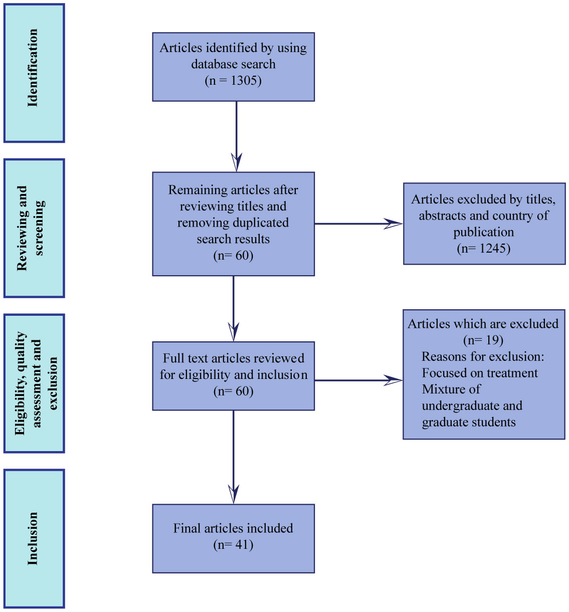
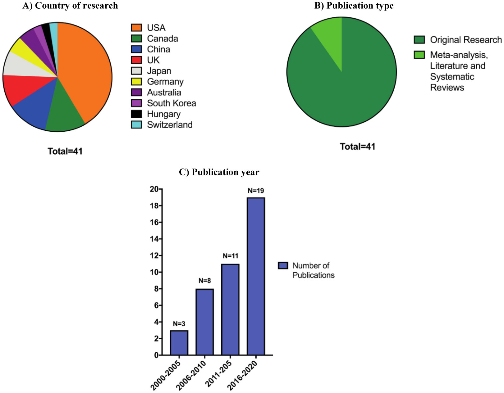
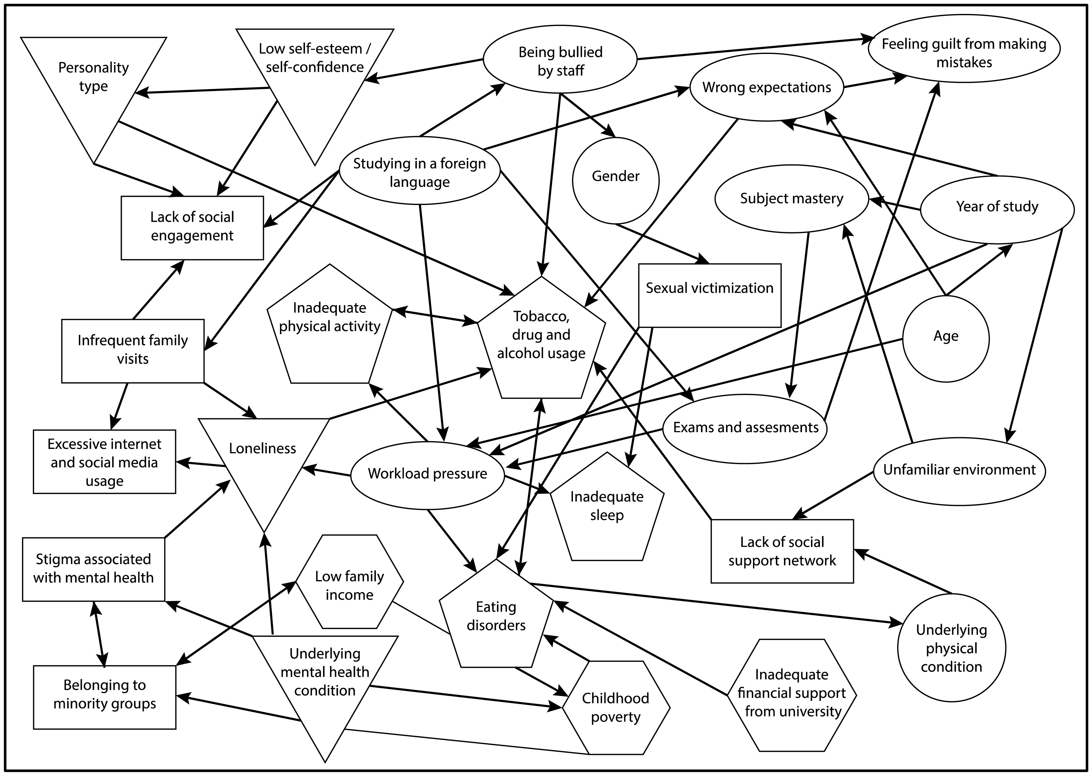
It is well-known that prevalence of stress, anxiety, and depression is high among university undergraduate students in developed and developing countries. Students entering university are from different socioeconomic background, which can bring a variety of mental health risk factors. The aim of this review was to investigate present literatures to identify risk factors associated with stress, anxiety, and depression among university undergraduate students in developed and developing countries. I identified and critically evaluated forty-one articles about risk factors associated with mental health of undergraduate university students in developed and developing countries from 2000 to 2020 according to the inclusion criteria. Selected papers were analyzed for risk factor themes. Six different themes of risk factors were identified: psychological, academic, biological, lifestyle, social and financial. Different risk factor groups can have different degree of impact on students' stress, anxiety, and depression. Each theme of risk factor was further divided into multiple subthemes. Risk factors associated with stress, depression and anxiety among university students should be identified early in university to provide them with additional mental health support and prevent exacerbation of risk factors.
- mental health,
- public health,
- stress,
- anxiety,
- depression,
- students,
- university,
- undergraduate
Citation: Mohammad Mofatteh. Risk factors associated with stress, anxiety, and depression among university undergraduate students[J]. AIMS Public Health, 2021, 8(1): 36-65. doi: 10.3934/publichealth.2021004

Related Papers:

Abstract

It is well-known that prevalence of stress, anxiety, and depression is high among university undergraduate students in developed and developing countries. Students entering university are from different socioeconomic background, which can bring a variety of mental health risk factors. The aim of this review was to investigate present literatures to identify risk factors associated with stress, anxiety, and depression among university undergraduate students in developed and developing countries. I identified and critically evaluated forty-one articles about risk factors associated with mental health of undergraduate university students in developed and developing countries from 2000 to 2020 according to the inclusion criteria. Selected papers were analyzed for risk factor themes. Six different themes of risk factors were identified: psychological, academic, biological, lifestyle, social and financial. Different risk factor groups can have different degree of impact on students' stress, anxiety, and depression. Each theme of risk factor was further divided into multiple subthemes. Risk factors associated with stress, depression and anxiety among university students should be identified early in university to provide them with additional mental health support and prevent exacerbation of risk factors.

Abbreviations

BDI

Beck's depression inventory

DSM

Diagnostic and statistical manual of mental disorders

PTSD

post-traumatic stress disorder

SAD

Stress, anxiety and depression

United Kingdom

USA

United States of America

Conflict of interest

All authors declare no conflicts of interest in this paper.

References

[1]	Pedrelli P, Nyer M, Yeung A, et al. (2015) College Students: Mental Health Problems and Treatment Considerations. Acad Psychiatry 39: 503-511. doi: 10.1007/s40596-014-0205-9
[2]	Mayer FB, Santos IS, Silveira PSP, et al. (2016) Factors associated to depression and anxiety in medical students: a multicenter study. BMC Med Educ 16: 282-282. doi: 10.1186/s12909-016-0791-1
[3]	Ibrahim AK, Kelly SJ, Adams CE, et al. (2013) A systematic review of studies of depression prevalence in university students. J Psychiatr Res 47: 391-400. doi: 10.1016/j.jpsychires.2012.11.015
[4]	Mkize LP, Nonkelela NF, Mkize DL (1998) Prevalence of depression in a university population. Curationis 21: 32-37.
[5]	Ivandic I, Kamenov K, Rojas D, et al. (2017) Determinants of Work Performance in Workers with Depression and Anxiety: A Cross-Sectional Study. Int J Environ Res Public Health 14: 466. doi: 10.3390/ijerph14050466
[6]	Ribeiro ÍJS, Pereira R, Freire IV, et al. (2018) Stress and Quality of Life Among University Students: A Systematic Literature Review. Health Professions Educ 4: 70-77. doi: 10.1016/j.hpe.2017.03.002
[7]	Ip EJ, Nguyen K, Shah BM, et al. (2016) Motivations and Predictors of Cheating in Pharmacy School. Am J Pharm Educ 80: 133-133. doi: 10.5688/ajpe808133
[8]	January J, Madhombiro M, Chipamaunga S, et al. (2018) Prevalence of depression and anxiety among undergraduate university students in low- and middle-income countries: a systematic review protocol. Syst Rev 7: 57. doi: 10.1186/s13643-018-0723-8
[9]	Whitton SW, Whisman MA (2010) Relationship satisfaction instability and depression US: American Psychological Association, 791-794.
[10]	Jackson-Koku G (2016) Beck Depression Inventory. Occup Med 66: 174-175. doi: 10.1093/occmed/kqv087
[11]	Ayuso-Mateos JL, Vázquez-Barquero JL, Dowrick C, et al. (2001) Depressive disorders in Europe: prevalence figures from the ODIN study. Brit J Psychiat 179: 308-316. doi: 10.1192/bjp.179.4.308
[12]	Gonzalez O, Berry J, McKnight-Eily LR, et al. (2010) Current Depression Among Adults—United States, 2006 and 2008. MMWR Morb Mortal Wkly Rep 59: 1229-1235.
[13]	Dyrbye LN, Thomas MR, Shanafelt TD (2005) Medical student distress: causes, consequences, and proposed solutions Mayo Clinic proceedings, Elsevier, 1613-1622.
[14]	Blanco C, Okuda M, Wright C, et al. (2008) Mental health of college students and their non-college-attending peers: results from the National Epidemiologic Study on Alcohol and Related Conditions. Arch Gen Psychiat 65: 1429-1437. doi: 10.1001/archpsyc.65.12.1429
[15]	Miron O, Yu KH, Wilf-Miron R, et al. (2019) Suicide Rates Among Adolescents and Young Adults in the United States, 2000–2017. JAMA 321: 2362-2364. doi: 10.1001/jama.2019.5054
[16]	Goodwill JR, Zhou S (2020) Association between perceived public stigma and suicidal behaviors among college students of color in the U.S.. J Affect Disord 262: 1-7. doi: 10.1016/j.jad.2019.10.019
[17]	Fergusson DM, Boden JM, Horwood LJ (2007) Recurrence of major depression in adolescence and early adulthood, and later mental health, educational and economic outcomes. Brit J Psychiat 191: 335-342. doi: 10.1192/bjp.bp.107.036079
[18]	UN DESA, United Nations Department of Economic and Social Affairs UN DESA, United Nations Department Of Economic And Social Affairs (2019) .Available from: https://www.un.org/development/desa/en/>.
[19]	Zivin K, Eisenberg D, Gollust SE, et al. (2009) Persistence of mental health problems and needs in a college student population. J Affect Disord 117: 180-185. doi: 10.1016/j.jad.2009.01.001
[20]	Turner AP, Hammond CL, Gilchrist M, et al. (2007) Coventry university students' experience of mental health problems. Couns Psychol Q 20: 247-252. doi: 10.1080/09515070701570451
[21]	Maser B, Danilewitz M, Guérin E, et al. (2019) Medical Student Psychological Distress and Mental Illness Relative to the General Population: A Canadian Cross-Sectional Survey. Acad Med 94. doi: 10.1097/ACM.0000000000002958
[22]	Ratanasiripong P, China T, Toyama S (2018) Mental Health and Well-Being of University Students in Okinawa. Educ Res Int 2018: 4231836. doi: 10.1155/2018/4231836
[23]	McCrae RR, John OP (1992) An introduction to the five-factor model and its applications. J Pers 60: 175-215. doi: 10.1111/j.1467-6494.1992.tb00970.x
[24]	Kawase E, Hashimoto K, Sakamoto H, et al. (2008) Variables associated with the need for support in mental health check-up of new undergraduate students. Psychiat Clin Neurosci 62: 98-102. doi: 10.1111/j.1440-1819.2007.01781.x
[25]	Fortney JC, Curran GM, Hunt JB, et al. (2016) Prevalence of probable mental disorders and help-seeking behaviors among veteran and non-veteran community college students. Gen Hosp Psychiat 38: 99-104. doi: 10.1016/j.genhosppsych.2015.09.007
[26]	Miller-Graff LE, Howell KH, Martinez-Torteya C, et al. (2015) Typologies of Childhood Exposure to Violence: Associations With College Student Mental Health. J Am Coll Health 63: 539-549. doi: 10.1080/07448481.2015.1057145
[27]	Wanda MC, Carla S (2013) Stress, Depression, and Anxiety among Undergraduate Nursing Students. Int J Nurs Educ Scholarship 10: 255-266. doi: 10.1515/ijnes-2012-0032
[28]	Ghodasara SL, Davidson MA, Reich MS, et al. (2011) Assessing Student Mental Health at the Vanderbilt University School of Medicine. Acad Med 86. doi: 10.1097/ACM.0b013e3181ffb056
[29]	Fares J, Al Tabosh H, Saadeddin Z, et al. (2016) Stress, Burnout and Coping Strategies in Preclinical Medical Students. North Am J Med Sci 8: 75-81. doi: 10.4103/1947-2714.177299
[30]	Macaskill A (2013) The mental health of university students in the United Kingdom. Brit J Guid Couns 41: 426-441. doi: 10.1080/03069885.2012.743110
[31]	Bovier PA, Chamot E, Perneger TV (2004) Perceived stress, internal resources, and social support as determinants of mental health among young adults. Qual Life Res 13: 161-170. doi: 10.1023/B:QURE.0000015288.43768.e4
[32]	Lee Kh, Ko Y, Kang Kh, et al. (2012) Mental Health and Coping Strategies among Medical Students. Korean J Med Educ 24: 55-63. doi: 10.3946/kjme.2012.24.1.55
[33]	Ishii T, Tachikawa H, Shiratori Y, et al. (2018) What kinds of factors affect the academic outcomes of university students with mental disorders? A retrospective study based on medical records. Asian J Psychiat 32: 67-72. doi: 10.1016/j.ajp.2017.11.017
[34]	Stallman HM (2010) Psychological distress in university students: A comparison with general population data. Aust Psychol 45: 249-257. doi: 10.1080/00050067.2010.482109
[35]	Scholz M, Neumann C, Ropohl A, et al. (2016) Risk factors for mental disorders develop early in German students of dentistry. Ann Anat Anat Anz 208: 204-207. doi: 10.1016/j.aanat.2016.06.004
[36]	Schweizer S, Kievit RA, Emery T, et al. (2018) Symptoms of depression in a large healthy population cohort are related to subjective memory complaints and memory performance in negative contexts. Psychol Med 48: 104-114. doi: 10.1017/S0033291717001519
[37]	Usher W, Curran C (2017) Predicting Australia's university students' mental health status. Health Promot Int 34: 312-322. doi: 10.1093/heapro/dax091
[38]	Call JB, Shafer K (2018) Gendered Manifestations of Depression and Help Seeking Among Men. Am J Mens Health 12: 41-51. doi: 10.1177/1557988315623993
[39]	Zeng W, Chen R, Wang X, et al. (2019) Prevalence of mental health problems among medical students in China: A meta-analysis. Medicine 98: e15337-e15337. doi: 10.1097/MD.0000000000015337
[40]	Brockelman KF (2009) The interrelationship of self-determination, mental illness, and grades among university students. J Coll Student Dev 50: 271-286. doi: 10.1353/csd.0.0068
[41]	Roberts SJ, Glod CA, Kim R, et al. (2010) Relationships between aggression, depression, and alcohol, tobacco: Implications for healthcare providers in student health. J Am Acad Nurse Pract 22: 369-375. doi: 10.1111/j.1745-7599.2010.00521.x
[42]	Cai L, Xu F, Cheng Q, et al. (2015) Social Smoking and Mental Health Among Chinese Male College Students. Am J Health Promot 31: 226-231. doi: 10.4278/ajhp.141001-QUAN-494
[43]	Tountas Y, Dimitrakaki C (2006) Health education for youth. Pediat Endocrinol Rev P 3: 222-225.
[44]	Tavolacci MP, Ladner J, Grigioni S, et al. (2013) Prevalence and association of perceived stress, substance use and behavioral addictions: a cross-sectional study among university students in France, 2009–2011. BMC Public Health 13: 724. doi: 10.1186/1471-2458-13-724
[45]	Boulton M, O'Connell KA (2017) Nursing Students' Perceived Faculty Support, Stress, and Substance Misuse. J Nurs Educ 56: 404-411. doi: 10.3928/01484834-20170619-04
[46]	Jenkins EK, Slemon A, O'Flynn-Magee K, et al. (2019) Exploring the implications of a self-care assignment to foster undergraduate nursing student mental health: Findings from a survey research study. Nurs Educ Today 81: 13-18. doi: 10.1016/j.nedt.2019.06.009
[47]	Rosenthal SR, Clark MA, Marshall BDL, et al. (2018) Alcohol consequences, not quantity, predict major depression onset among first-year female college students. Addict Behav 85: 70-76. doi: 10.1016/j.addbeh.2018.05.021
[48]	Terebessy A, Czeglédi E, Balla BC, et al. (2016) Medical students' health behaviour and self-reported mental health status by their country of origin: a cross-sectional study. BMC Psychiat 16: 171. doi: 10.1186/s12888-016-0884-8
[49]	Wallace DD, Boynton MH, Lytle LA (2017) Multilevel analysis exploring the links between stress, depression, and sleep problems among two-year college students. J Am Coll Health 65: 187-196. doi: 10.1080/07448481.2016.1269111
[50]	Hefner J, Eisenberg D (2009) Social support and mental health among college students. Am J Orthopsychiat 79: 491-499. doi: 10.1037/a0016918
[51]	Meng X, Kou C, Shi J, et al. (2011) Susceptibility genes, social environmental risk factors and their interactions in internalizing disorders among mainland Chinese undergraduates. J Affect Disord 132: 254-259. doi: 10.1016/j.jad.2011.01.005
[52]	Whitton SW, Weitbrecht EM, Kuryluk AD, et al. (2013) Committed Dating Relationships and Mental Health Among College Students. J Am Coll Health 61: 176-183. doi: 10.1080/07448481.2013.773903
[53]	Michalec B, Keyes CLM (2013) A multidimensional perspective of the mental health of preclinical medical students. Psychol Health Med 18: 89-97. doi: 10.1080/13548506.2012.687825
[54]	McDougall EE, Langille DB, Steenbeek AA, et al. (2016) The Relationship Between Non-Consensual Sex and Risk of Depression in Female Undergraduates at Universities in Maritime Canada. J Interpers Violence 34: 4597-4619. doi: 10.1177/0886260516675468
[55]	Yao B, Han W, Zeng L, et al. (2013) Freshman year mental health symptoms and level of adaptation as predictors of Internet addiction: a retrospective nested case-control study of male Chinese college students. Psychiat Res 210: 541-547. doi: 10.1016/j.psychres.2013.07.023
[56]	Thomas L, Orme E, Kerrigan F (2020) Student Loneliness: The Role of Social Media Through Life Transitions. Comput Educ 146: 103754. doi: 10.1016/j.compedu.2019.103754
[57]	Li M, Li WQ, Li LMW (2019) Sensitive Periods of Moving on Mental Health and Academic Performance Among University Students. Front Psychol 10: 1289. doi: 10.3389/fpsyg.2019.01289
[58]	Sznitman SR, Reisel L, Romer D (2011) The Neglected Role of Adolescent Emotional Well-Being in National Educational Achievement: Bridging the Gap Between Education and Mental Health Policies. J Adolesc Health 48: 135-142. doi: 10.1016/j.jadohealth.2010.06.013
[59]	Vaughn AA, Drake RR, Haydock S (2016) College student mental health and quality of workplace relationships. J Am Coll Health 64: 26-37. doi: 10.1080/07448481.2015.1064126
[60]	Bradley G (2000) Responding effectively to the mental health needs of international students. High Educ 39: 417-433. doi: 10.1023/A:1003938714191
[61]	Park SY, Andalibi N, Zou Y, et al. (2020) Understanding Students' Mental Well-Being Challenges on a University Campus: Interview Study. JMIR Form Res 4: e15962. doi: 10.2196/15962
[62]	Brown JSL (2018) Student mental health: some answers and more questions. J Ment Health 27: 193-196. doi: 10.1080/09638237.2018.1470319
[63]	Armstrong LL, Young K (2015) Mind the gap: Person-centred delivery of mental health information to post-secondary students. Psychosoc Interv 24: 83-87. doi: 10.1016/j.psi.2015.05.002
[64]	Erschens R, Keifenheim KE, Herrmann-Werner A, et al. (2019) Professional burnout among medical students: Systematic literature review and meta-analysis. Med Teach 41: 172-183. doi: 10.1080/0142159X.2018.1457213
[65]	Hafen M, Reisbig AMJ, White MB, et al. (2006) Predictors of Depression and Anxiety in First-Year Veterinary Students: A Preliminary Report. J Vet Med Educ 33: 432-440. doi: 10.3138/jvme.33.3.432
[66]	Hunt J, Eisenberg D (2010) Mental Health Problems and Help-Seeking Behavior Among College Students. J Adolesc Health 46: 3-10. doi: 10.1016/j.jadohealth.2009.08.008
[67]	Kitzrow MA (2003) The Mental Health Needs of Today's College Students: Challenges and Recommendations. NASPA J 41: 167-181. doi: 10.2202/0027-6014.1310
[68]	Sprung JM, Rogers A (2020) Work-life balance as a predictor of college student anxiety and depression. J Am Coll Health 1-8. doi: 10.1080/07448481.2019.1706540

Reader Comments

Your name:*

Email:*
© 2021 the Author(s), licensee AIMS Press. This is an open access article distributed under the terms of the Creative Commons Attribution License (http://creativecommons.org/licenses/by/4.0)