Review Special Issues

A review of ultrasound detection methods for breast microcalcification

  • Breast microcalcifications are one of the important imaging features of early breast cancer and are a key to early breast cancer diagnosis. Ultrasound imaging has been widely used in the detection and diagnosis of breast diseases because of its low cost, nonionizing radiation, and real-time capability. However, due to factors such as limited spatial resolution and speckle noise, it is difficult to detect breast microcalcifications using conventional B-mode ultrasound imaging. Recent studies show that new ultrasound technologies improved the visualization of microcalcifications over conventional B-mode ultrasound imaging. In this paper, a review of the literature on the ultrasonic detection methods of microcalcifications was conducted. The reviewed methods were broadly divided into high-frequency B-mode ultrasound imaging techniques, B-mode ultrasound image processing techniques, ultrasound elastography techniques, time reversal techniques, high spatial frequency techniques, second-order ultrasound field imaging techniques, and photoacoustic imaging techniques. The related principles and research status of these methods were introduced, and the characteristics and limitations of the various methods were discussed and analyzed. Future developments of ultrasonic breast microcalcification detection are suggested.

    Citation: Yali Ouyang, Zhuhuang Zhou, Weiwei Wu, Jin Tian, Feng Xu, Shuicai Wu, Po-Hsiang Tsui. A review of ultrasound detection methods for breast microcalcification[J]. Mathematical Biosciences and Engineering, 2019, 16(4): 1761-1785. doi: 10.3934/mbe.2019085

    Related Papers:

    [1] Lorenza D'Elia . Γ-convergence of quadratic functionals with non uniformly elliptic conductivity matrices. Networks and Heterogeneous Media, 2022, 17(1): 15-45. doi: 10.3934/nhm.2021022
    [2] Andrea Braides, Valeria Chiadò Piat . Non convex homogenization problems for singular structures. Networks and Heterogeneous Media, 2008, 3(3): 489-508. doi: 10.3934/nhm.2008.3.489
    [3] Patrick Henning . Convergence of MsFEM approximations for elliptic, non-periodic homogenization problems. Networks and Heterogeneous Media, 2012, 7(3): 503-524. doi: 10.3934/nhm.2012.7.503
    [4] Leonid Berlyand, Volodymyr Rybalko . Homogenized description of multiple Ginzburg-Landau vortices pinned by small holes. Networks and Heterogeneous Media, 2013, 8(1): 115-130. doi: 10.3934/nhm.2013.8.115
    [5] Manuel Friedrich, Bernd Schmidt . On a discrete-to-continuum convergence result for a two dimensional brittle material in the small displacement regime. Networks and Heterogeneous Media, 2015, 10(2): 321-342. doi: 10.3934/nhm.2015.10.321
    [6] Fabio Camilli, Claudio Marchi . On the convergence rate in multiscale homogenization of fully nonlinear elliptic problems. Networks and Heterogeneous Media, 2011, 6(1): 61-75. doi: 10.3934/nhm.2011.6.61
    [7] Brahim Amaziane, Leonid Pankratov, Andrey Piatnitski . Homogenization of variational functionals with nonstandard growth in perforated domains. Networks and Heterogeneous Media, 2010, 5(2): 189-215. doi: 10.3934/nhm.2010.5.189
    [8] Antonio DeSimone, Martin Kružík . Domain patterns and hysteresis in phase-transforming solids: Analysis and numerical simulations of a sharp interface dissipative model via phase-field approximation. Networks and Heterogeneous Media, 2013, 8(2): 481-499. doi: 10.3934/nhm.2013.8.481
    [9] Liselott Flodén, Jens Persson . Homogenization of nonlinear dissipative hyperbolic problems exhibiting arbitrarily many spatial and temporal scales. Networks and Heterogeneous Media, 2016, 11(4): 627-653. doi: 10.3934/nhm.2016012
    [10] Peter Bella, Arianna Giunti . Green's function for elliptic systems: Moment bounds. Networks and Heterogeneous Media, 2018, 13(1): 155-176. doi: 10.3934/nhm.2018007
  • Breast microcalcifications are one of the important imaging features of early breast cancer and are a key to early breast cancer diagnosis. Ultrasound imaging has been widely used in the detection and diagnosis of breast diseases because of its low cost, nonionizing radiation, and real-time capability. However, due to factors such as limited spatial resolution and speckle noise, it is difficult to detect breast microcalcifications using conventional B-mode ultrasound imaging. Recent studies show that new ultrasound technologies improved the visualization of microcalcifications over conventional B-mode ultrasound imaging. In this paper, a review of the literature on the ultrasonic detection methods of microcalcifications was conducted. The reviewed methods were broadly divided into high-frequency B-mode ultrasound imaging techniques, B-mode ultrasound image processing techniques, ultrasound elastography techniques, time reversal techniques, high spatial frequency techniques, second-order ultrasound field imaging techniques, and photoacoustic imaging techniques. The related principles and research status of these methods were introduced, and the characteristics and limitations of the various methods were discussed and analyzed. Future developments of ultrasonic breast microcalcification detection are suggested.


    Natural hazards such as landslides and subsidence have been recognized as important impediments to developing nations' sustainable development [1,2,3,4]. For example, on December 20, 2015, in Guangming, Shenzhen, China, a catastrophic landfill slope landslide claimed the lives of 69 individuals [5]. Natural hazard risk assessment and management will have short-term benefits in terms of severity reduction and long-term benefits in terms of achieving sustainable development goals [1].

    Slope stability evaluation is essential for analyzing and mitigating natural hazards in mountainous environments. Many attempts have been made to evaluate slope stability [6,7,8]. Owing to the inherent complexity and uncertainty, assessing slope stability for circular mode failure, a common problem, remains a challenge for practitioners and researchers [9]. Several methods for evaluating slope stability have been presented, with the limit equilibrium approach and numerical simulation method being the two most commonly used [10]. Limited equilibrium methods, such as the simplified Bishop, Spencer and Morgenstern-Price methods, are frequently implemented in practice. In general, soil material properties (unit weight, cohesion and friction angle) and the pore pressure ratio are required for limited equilibrium methods [11,12]. Numerical methods (e.g., finite element methods) have been extensively used to analyze slope stability. However, the major drawback is that their input parameters need to be back analyzed using in-situ measurements, which is not available in many cases [13]. Both methods have pros and cons. Finding the critical slip surface using the limit equilibrium method is difficult due to the large number of potential slip surfaces [14]. The numerical simulation method's accuracy is greatly influenced by the choice of constitutive models, mechanical parameters and boundary conditions, and it is frequently necessary to have a great deal of engineering expertise and to conduct on-site back analysis in order to make a reasonable choice and obtain reasonable results [15,16]. Consequently, predicting slope stability still presents considerable challenges.

    In recent years, machine learning (ML) models have gained attention for solving very complex, nonlinear and multivariable geotechnical problems [17,18,19]. Assessments of slope stability circular failure using methods based on soft computing are summarized in Table 1. Despite their reliable and precise outputs, however, most algorithms are not readily applicable in practice owing to their complicated training and modeling procedures and "black box" aspects, i.e., these models do not demonstrate a transparent and understandable relationship between inputs and output. Quinlan [20] developed the model tree algorithm to get over these limitations. It integrates principles from decision trees and linear regression. In addition to the widespread application of soft computing techniques, several studies have only been conducted on a limited amount of data, which might restrict the classifier's ability to generalize. In the current study, an updated database of 627 cases comprising unit weight, cohesion, internal friction angle, slope angle and height, pore pressure ratio and stability status of circular mode failure has been compiled. To predict slope stability, a new logistic model tree (LMT) model is developed. This algorithm is an intelligent choice for classification and decision-making since it can solve the classification problem by combining a tree model and a logistic regression (LR) technique. Adding LR to the leaves of the tree allows for a probabilistic interpretation of the model's output, making it easier to explain, as they represent a series of if-then-else rules. The LMT has been employed in predicting pillar stability in geotechnical engineering [21], but it has not yet been used to predict slope stability.

    Table 1.  A summary of the ML-based circular mode failure assessment of slope stability.
    Dataset (Stable/Failed) Input parameters Data Preprocessing ML techniques Reference
    422 (226/196) γ, c, ϕ, β, H, ru Data normalization MDMSE Zhang et al. [22]
    444 (224/220) γ, c, ϕ, β, H, ru Data normalization AdaBoost, GBM Bagging, XRT, RF, HGB Voting Stacked Lin et al. [23]
    19 (13/6) γ, c, ϕ, β, H, ru Data normalization K-means cluster Haghshenas et al. [24]
    153 (83/70) γ, c, ϕ, β, H, ru Data normalization and outlier removing KNN, SVM, SGD, GP, QDA, GNB, DT, ANN, Bagging ensemble, Heterogeneous ensemble Pham et al. [25]
    257 (123/134) γ, c, ϕ, β, H, ru XGB, RF, LR, SVM, BC, LDA, KNN, DT, MLP, GNB, XRT, Stacked ensemble Kardani et al. [26]
    87 (42/45) γ, c, ϕ, β, H, ru J48 Amirkiyaei and Ghasemi [27]
    221 (115/106) γ, c, ϕ, β, H, ru Data normalization ANN, SVM, RF, GBM Zhou et al. [28]
    148 (78/70) γ, c, ϕ, β, H, ru Data normalization LR, DT, RF, GBM, SVM, BP Qi and Tang [29]
    168 (84/84) γ, c, ϕ, β, H, ru Data normalization GP, QDA, SVM, ADB-DT, ANN, KNN Classifier ensemble Qi and Tang [15]
    107 (48/59) γ, c, ϕ, β, H, ru RF, SVM, Bayes, GSA Lin et al. [30]
    82 (49/33) γ, c, ϕ, β, H, ru NB Feng et al. [31]
    168 (84/84) γ, c, ϕ, β, H, ru Data normalization RBF, LSSVM, ELM Hoang and Bui [32]
    168 (84/84) γ, c, ϕ, β, H, ru Data normalization LSSVM Hoang and Pham [33]
    46 (17/29) γ, c, ϕ, β, H, ru Data normalization SVM Xue et al. [34]
    32 (14/18) γ, c, ϕ, β, H, ru ANN Lu and Rosenbaum [35]
    82 (38/44) γ, c, ϕ, β, H, ru BP Feng [36]
    Note: MDMSE-margin distance minimization selective ensemble, AdaBoost-adaptive boosting, GBM-gradient boosting machine, XRT-extremely randomized tree, RF-random forest, HGB-hist gradient boosting classifier, KNN-k-nearest neighbors, SVM-support vector machine, SGD-stochastic gradient descent, GP-Gaussian process, QDA-quadratic discriminant analysis, GNB-Gaussian naive Bayes, DT-decision tree, ANN-artificial neural network, XGB-extreme gradient boosting, BC-bagging classifier, LDA-linear discriminant analysis, MLP-multilayer perceptron, BP-back-propagation, QDA-quadratic discriminant analysis, ADB-DT-adaptive boosted decision tree, GSA-gravitational search algorithm, NB-naive Bayes, RBF-radial basis function, LSSVM-least squares support vector machine, ELM-extreme learning machine, γ-unit weight, c-cohesion, ϕ-angle of internal friction, β-slope angle, H-slope height, ru-pore pressure ratio.

     | Show Table
    DownLoad: CSV

    LR is a straightforward method with features such as stability, low variance and time-efficient training [37], but its prediction outputs are frequently biased. Decision trees are another ML technique for searching a less confined space of candidate models and obtaining nonlinear patterns from a database; they have low bias but high variance and instability, making them susceptible to overfitting. Landwehr et al. [38] presented the LMT methodology as a result. It is based on Quinlan's model tree approach [20] for dealing with regression problems by combining linear regression with decision tree models, and it is extended to classification problems. This section provides a basic introduction to LMT, whereas the seminal work by Landwehr et al. [38] provides a more complete description.

    A LR tree with LR functions built at the leaves constitutes an LMT. It has a set of leaves or terminal nodes T and an inner or non-terminal node set N. Each leaf t of the LMT model has correlated LR functions instead of classification labels or linear regression functions. The output vector is Y, and the input vector X is (X1, X2), for instance. S represents the complete instance space, which can be further partitioned into numerous subspaces St. Figure 1 displays a simple input space that has been partitioned into seven subspaces.

    Figure 1.  The input space is separated into seven subspaces (solid circles and square points represent different classes within the same case, and each subspace has its own function).
    S=tTSt,StSt= (1)

    The model determines LR functions for the seven subspaces represented in Figure 1. Figure 2 depicts the structure of the tree.

    Figure 2.  Example of a simplified LMT structure corresponding to the sample data shown in Figure 1 (adapted from Landwehr et al. [38]).

    In contrast to standard forms of LR, the LogitBoost technique for fitting additive LR models proposed by Friedman et al. [39] is employed for model construction here. The prediction probability is given by Eq (2).

    Pr(G=j|X=x)=eFj(x)Jk=1eFk(x) (2)

    where G denotes the output, J denotes the class labels, X denotes the inputs, and Fj(x) denotes the functions that the LMT will train in the tree's leaves, as follows:

    Fj(x)=Mm=1fmj(x)=αj0+SStαjSS (3)

    where m is the number of iterations, fmj represents the functions of input variables, α represents the intercepts and coefficients of the linear function, and S represents the variables of the subset St at the leaf t.

    A LMT can be established by the following steps: initial tree growth, tree splitting and stopping, and tree pruning. This section presents the basic idea; the reader is referred to Landwehr et al. [38] for additional detail. The M5P technique, which is commonly used for tree growth, can first construct a standard tree, after which a LR model can be established at each node [40,41]. This technique merely trains the model using case histories at each node in isolation, without taking the surrounding tree structure into account; therefore, in order for the LogitBoost algorithm to iteratively change Fj(x) to increase the fit in a natural way, another technique-one that can incrementally refine logistic model fit at high levels-is used [38]. The function fmj is introduced to Fj by changing one of the function's coefficients or introducing another variable (see Eq (3)). As a result, in the initial growing process, a LR tree is formed in the root using proper iteration numbers. The tree then begins to grow by resembling specified subsets (t) from the database (S) to the child nodes, utilizing the C4.5 splitting law [20] to increase the accuracy of the classification variable. The LR functions are generated in the child nodes by running the LogitBoost algorithm with the logistic model, weights and probability estimate from the previous iteration at the parent node. The splitting process is then repeated. When it comes to model fitting, the tree stops splitting when a node has less than 15 cases. After the tree is constructed, the tree pruning approach is used to trade off tree size and model complexity while maintaining predictive accuracy. After experimenting with several pruning initiatives, Landwehr et al. [38] employed the classification and regression trees pruning approach [42] to make pruning decisions while taking training error and model complexity into account. These three processes can be used to create a LMT.

    An updated database with 627 instances was obtained from previous studies [22,23,25,29,33,43] and can be found in Table S1 of the supplementary information file. The database includes the unit weight, cohesion, angle of internal friction, slope angle and height, pore pressure ratio and slope stability status. There are 311 positive (stable) and 316 negative (failed) samples. The statistics of the input features are summarized in Table 2. The data normalization is not carried out owing to the fact that tree-based methods are insensitive to feature scaling; they make decisions based on relative feature values and splits [44]. The database box plot is shown in Figure 3, where solid black spots represent "outliers", and the statistical features are shown in Table 2. The bottom and top quartiles are shown by horizontal lines, while the median values are represented by bold lines inside the boxes. Slopes with "failed" and "stable" instances are also demonstrated separately.

    Table 2.  Statistical values for features in the database.
    Input parameter Unit Min. Max. Mean Std. Dev.
    Unit weight (γ) kN/m3 0.492 33.16 20.185 7.044
    Cohesion (c) kPa 0 300 25.6 31.036
    Angle of internal friction (ϕ) 0 49.5 25.308 12.331
    Slope angle (β) 0.302 65 32.605 13.711
    Slope height (H) m 0.018 565 90.289 120.14
    Pore pressure ratio (ru) 0 1 0.254 0.26

     | Show Table
    DownLoad: CSV
    Figure 3.  Box plots show the variation among data points in the database.

    The classification metrics include accuracy evaluation indices (accuracy (Acc), Matthews correlation coefficient (Mcc), precision (Prec), recall (Rec) and F-score) that are calculated from the confusion matrix (see Figure 4).

    Figure 4.  Confusion matrix (2 × 2) for classification problem.

    Each row of the matrix represents the instances in an actual class, while each column represents the instances in a predicted class [45]. In predictive analytics, a confusion matrix is described as a table with two rows and two columns that provides the numbers of true positives (TPs), true negatives (TNs), false positives (FPs) and false negatives (FNs). The classification evaluation metrics derived from the confusion matrix results were used to compare the prediction performances of the models [46,47,48]:

    Acc=TN+TPTN+FP+FN+TP (4)
    Prec=TNFN+TNorTPTP+FP (5)
    Rec=TNTN+FPorTPTP+FN (6)
    Fscore=21Precision+1Recall (7)
    Mcc=TN×TPFP×FN(FN+TP)(FP+TN)(FP+TP)(FN+TN) (8)

    Acc is the sum of TP and TN and represents the percentage of correctly classified instances in the data as a whole. This metric measures the model's total prediction accuracy. If the data set is unbalanced, that is, the numbers of observations in different classes vary substantially, accuracy will be deceiving [49]. As a result, further assessment metrics such as precision, recall, F-score and Mcc were utilized to examine the model's performance further. Precision is known as positive predicted value, and recall is known as true positive rate (TPR). F-score is a generalized index that evaluates the performance of both recall and precision and ranges from 0 (worst value) to 1 (best value). Mcc denotes the degree of agreement between observed and predicted classes of failed and stable instances [48]. It is a standard metric used by statisticians that accepts values ranging from −1 to 1. Mcc value of −1 indicates complete disagreement (strong negative association), a value of 1 indicates complete agreement (strong positive association), and a value of 0 indicates that the prediction was unrelated to the ground truth (very weak or no correlation between dependent and independent variables). Additionally, another succinct metric, i.e., area under the receiver operating characteristic curve (AUC), was employed for effective evaluation. This curve is expressed in a graphical plot that shows a binary classification system's diagnostic capacity as its discrimination threshold changes. The AUC is plotted by comparing the TPR vs. the false positive rate (FPR) at various threshold levels. An acceptable classification model should have an AUC near to 1. Table 3 shows the main rule for defining discrimination based on AUC value [25].

    Table 3.  Rule for classifying discrimination based on AUC value.
    Discrimination category AUC value
    No discrimination AUC = 0.5
    Acceptable 0.7 ≤ AUC < 0.8
    Excellent 0.8 ≤ AUC < 0.9
    Outstanding 0.9 ≤ AUC

     | Show Table
    DownLoad: CSV

    Waikato Environment for Knowledge Analysis (WEKA) software was used for developing a model based on the acquired data set. WEKA is a collection of ML algorithms that supports data mining tasks by providing a wide range of tools that can be used for data pre-processing, classification, clustering, regression, association and visualization [50]. The database was divided into two parts: training (80%) and testing (20%). The training set contained 249 stable instances and 253 failed cases, while the test set contained 125 instances, 62 of which were stable and 63 of which were failed instances. The stable-to-failed instance ratios in the training and testing sets were close to one, indicating that the distribution of these two instances does not necessitate a cost-sensitive technique to address problem due to imbalance [51,52].

    Every terminal node (or leaf) of the tree model was trained and updated using LR models during training (see Section 2). The minimal number of instances for the LMT model was determined to be 15 based on predictive performance, readily applicable tree structure and total training data. The size of the tree was 45, and it had 23 leaves. LogitBoost had a weight trimming value of 0.2 and a number of iterations of −1. Figure 5 depicts a representation of a tree generated by LMT. The LMT model has 23 logistic functions (LMs), and their detailed expressions are shown in Table 4. It is important to notice that some of the functions in Table 4 do not incorporate all of the parameters that have been chosen. The LM1 function for stable slopes in Table 4, for example, does not account for unit weight (γ). The simple logistic technique is used in the LMT training phase [38]. The goal of the simple logistic method is to control the parameter numbers as simply and straightforwardly as possible. New parameters are gradually introduced during training in order to improve the performance of each function at each node of the tree (see Section 2). This can also help to avoid the issue of model significance in LR, especially when using multiple logistic functions to build a full logistic model with all parameters. However, just a few of the functions had fewer parameters than those selected, showing that most of the factors we chose have an influence on predictive performance.

    Figure 5.  A LMT's structure.
    Table 4.  Logistic functions in the LMT model.
    No. Regression model for the slope stability condition No. Regression model for the slope stability condition
    LM1 FS=0.3+14.53c+4.62ϕ5.83β9.17H0.69ru
    FF=0.314.53c4.62ϕ+5.83β+9.17H+0.69ru
    LM13 FS=1.870.01c0.03ϕ+0.04β+0H+1.3ru
    FF=1.87+0.01c+0.03ϕ0.04β0H1.3ru
    LM2 FS=0.360.04γ+0.02c0.04ϕ+0.13β0.05H
    FF=0.36+0.04γ0.02c+0.04ϕ0.13β+0.05H
    LM14 FS=6.73+0.22γ0.01c0.03ϕ+0.05β0H+1.3ruFF=6.730.22γ+0.01c+0.03ϕ0.05β+0H1.3ru
    LM3 FS=0.730.07γ0.02c0.13ϕ+0.11β+0.08H+3.03ru
    FF=0.73+0.07γ+0.02c+0.13ϕ0.11β0.08H3.03ru
    LM15 FS=10.690.01c0.09ϕ+0.28β+0H+2.97ruFF=10.69+0.01c+0.09ϕ0.28β0H2.97ru
    LM4 FS=5.08+0.02γ0.02c0.1ϕ+0.28β+0H8.66ru
    FF=5.080.02γ+0.02c+0.1ϕ0.28β0H+8.66ru
    LM16 FS=8.310.01c+0.02ϕ+0.02β+0H1.59ruFF=8.31+0.01c0.02ϕ0.02β0H+1.59ru
    LM5 FS=7.18+0.01γ0.01c0.04ϕ+0β
    FF=7.180.01γ+0.01c+0.04ϕ0β
    LM17 FS=2.050.01c+0.02ϕ+0.02β+0H1.67ru
    FF=2.05+0.01c0.02ϕ0.02β0H+1.67ru
    LM6 FS=4.40.51γ+0.03ϕ+0.09β+0.01H
    FF=4.4+0.51γ0.03ϕ0.09β0.01H
    LM18 FS=7.6+0.2γ0.04c0.1ϕ0.01β0.08H1.42ruFF=7.60.2γ+0.04c+0.1ϕ+0.01β+0.08H+1.42ru
    LM7 FS=27.081.49γ0.09c0.17ϕ0.22β0.02H+23.63ru
    FF=27.08+1.49γ+0.09c+0.17ϕ+0.22β+0.02H23.63ru
    LM19 FS=4.4+0.58γ0.04c0.07ϕ0.01β+0.01H1.72ru
    FF=4.40.58γ+0.04c+0.07ϕ+0.01β0.01H+1.72ru
    LM8 FS=9.31+0.08γ0.03c+0.01ϕ+0.03β0H+0.31ru
    FF=9.310.08γ+0.03c0.01ϕ0.03β+0H0.31ru
    LM20 FS=5.13+0.25γ0.11c0.05ϕ+0.08β0.01H+5.74ru
    FF=5.130.25γ+0.11c0.05ϕ0.08β+0.01H5.74ru
    LM9 FS=11.33+0.03γ+0.02c0.04ϕ0.31β+0.02H23.05ru
    FF=11.330.03γ0.02c+0.04ϕ+0.31β0.02H+23.05ru
    LM21 FS=10.75+0.74γ0c0.16ϕ+0.09β0H2.68ru
    FF=10.750.74γ+0c+0.16ϕ0.09β+0H+2.68ru
    LM10 FS=4.750.21γ0.01c0.06ϕ+0.07β+0H2.67ru
    FF=4.75+0.21γ+0.01c+0.06ϕ0.07β0H+2.67ru
    LM22 FS=90.05+1.93γ0.01c+0.41ϕ+0.48β+0H+0.58ru
    FF=90.051.93γ+0.01c0.41ϕ0.48β0H0.58ru
    LM11 FS=0.170.01γ+0c+0.02ϕ+0β1.67ru
    FF=0.17+0.01γ0c0.02ϕ0β+1.67ru
    LM23 FS=98.1+2.52γ+0.86c1.19ϕ0β+0.01H+3.15ru
    FF=98.12.52γ0.86c+1.19ϕ+0β0.01H3.15ru
    LM12 FS=43.040.01γ+0c+0.73ϕ0.2β+43.7ru
    FF=43.04+0.01γ0c0.73ϕ+0.2β43.7ru
    Note: Angle of internal friction (ϕ) and slope angle (β) are in degrees.

     | Show Table
    DownLoad: CSV

    The proposed LMT model was quantified using several performance metrics based on confusion matrices. The confusion matrices of the model in training and test sets were then obtained, as shown in Table 5.

    Table 5.  Confusion matrices and performance metric results for training and testing datasets.
    Dataset Actual Predicted Acc (%) Mcc AUC Prec Rec F-score
    Stable Failed
    Training Stable 237 12 92.23 0.846 0.974 0.898 0.952 0.924
    Failed 27 226 0.950 0.893 0.921
    Testing Stable 51 11 85.60 0.713 0.907 0.879 0.823 0.850
    Failed 7 56 0.836 0.889 0.862

     | Show Table
    DownLoad: CSV

    The proposed LMT model predicts two classes (stable and failed). Table 5 displays the confusion matrices that illustrate training and prediction results. The number of cases that could have been correctly predicted is indicated by the values along the major diagonal. The results of Table 5 show that the LMT correctly classified the majority of the cases.

    The prediction outcomes of classification problems can be assessed using a variety of metrics, such as Acc, Mcc, AUC, recall, precision and F-score. The LMT model performed well in both the training set (Acc = 92.23%, Mcc = 0.846, AUC = 0.974, F-score for stable state = 0.924 and F-score for failed state = 0.921) and testing set (Acc = 85.60%, Mcc = 0.713, AUC = 0.907, F-score for stable state = 0.850 and F-score for failed state = 0.862). The employed metrics show that the prediction's results are accurate and acceptable.

    The LMT model achieved better prediction performance (Acc = 0.856 and AUC = 0.907) in comparison to the SVM model (Acc = 0.812 and AUC = 0.796), SGD model (Acc = 0.640 and AUC = 0688), QDA model (Acc = 0.788 and AUC = 0.817), GNB model (Acc = 0.812 and AUC = 0.775), DT model (Acc = 0.788 and AUC = 0.829) and RT model (Acc = 0.788 and AUC = 0.904), reported by Pham et al. [25], respectively, for the test data. When using ML techniques to predict slope stability, Acc generally ranges from 0.640 to 0.812, according to the results of previous study by Pham et al. [25]. Meanwhile, in the present study, it is 0.856 for the test data set. However, due to the use of different data sets, a comparison between these results is unwarranted. A project that uses different data sets is needed to give a generalized model to predict slope stability. Additionally, the results for relatively small sample sizes (less than 100) are not presented or compared. These comparative results demonstrate conclusively that the LMT model is capable of improved generalization performance compared to other models in the literature. The potential reasons underlying this observation are that the LMT model can capture interactions between features effectively, the branching structure of the decision tree can identify feature interactions, and LR at the leaves can model the relationships between these interactions and the target variable.

    Two case studies are analyzed using our proposed LMT-based slope stability prediction model to determine its efficacy and applicability in engineering practice. The LMT model predicted ten slope stability status events in two different projects. The field data was obtained from the available literature, which includes the Shao Jiazhuang slope failure [53] and the Daguangbao landslide [54].

    The slope at Shao Jiazhuang village in Guizhou province, China (see Figure 6 (a)) [53], is utilized as a real-world example to analyze slope stability with the proposed LMT model and validate its efficacy and practicality in engineering practice application. As depicted in Figure 6(c)(e), during the survey, there were localized shallow surface collapses and new cracks on the slope's left side [53].

    Figure 6.  Slope failure area at Shao Jiazhuang, China: (a) location map, (b) slope collapse, (c), (d) collapse zone, and (e) crack.

    The input data shown in Table 6 were used by the LMT to predict the stability of the case slope based on the material parameters and geometry feature parameters of the case slope. The slope is failed, according to the prediction's outcome. This study demonstrates that the LMT model is reliable for predicting slope stability and that it can be applied to a variety of geotechnical applications.

    Table 6.  Application of the proposed LMT model in real-world slope stability prediction.
    S. No. γ (kN/m3) c (kPa) ϕ (°) β (°) H (m) ru Actual status LMT predicted result
    1 20 22.4 28 39.47 14 0 Failed Failed

     | Show Table
    DownLoad: CSV

    The Daguangbao landslide, is one of the few extremely big landslides known to exist worldwide, with a size of over 1 billion m3 [55]. It is also the most extensive and largest landslide ever recorded in Chinese historical records. Because of its massive volume, unusual genetic mechanism and complex movement process [56,57,58], the Daguangbao landslide has drawn a lot of attention and interest.

    The stability evaluation is carried out on 9 slopes, approved by specialists, from the Daguangbao landslide, of which 5 are stable, and 4 failed [54]. The index values of the samples and predicted results of the LMT model are compared to the fuzzy discriminant method and the unascertained measure method in Table 7.

    Table 7.  Predicted results using LMT, fuzzy discriminant and unascertained measure methods.
    S. No. γ (kN/m3) c (kPa) ϕ (°) β (°) H (m) ru Actual status LMT proposed method Fuzzy discriminant method [54] Unascertained measure method [54]
    1 27 32 33 42.4 289 0.25 Stable Stable Stable Stable
    2 20.41 33 11 16 46 0.2 Failed Failed Stable* Failed
    3 21.43 0 20 20 61 0.5 Failed Failed Failed Failed
    4 19.63 11.97 20 22 21.19 0.405 Failed Failed Failed Failed
    5 18.68 26.34 15 35 8.23 0.25 Failed Failed Failed Stable*
    6 27 50 40 42 407 0.25 Stable Stable Stable Stable
    7 27.3 14 31 50 92 0.25 Stable Stable Stable Failed*
    8 21.4 10 30.34 30 20 0.25 Stable Stable Stable Stable
    9 25 46 35 46 393 0.25 Stable Stable Stable Stable
    Note: (*) wrongly predicted.

     | Show Table
    DownLoad: CSV

    The prediction outcomes in Table 7 indicate that the slope stability was predicted correctly for all cases. The theory of unascertained measure and its mathematical processing were first put forward by Wang [59] in 1990. On this basis, Liu et al. [60,61] established the unascertained mathematical theory and applied it to decision-making problems. Unascertained information is a new kind of uncertainty information which is different from fuzzy information, random information and grey information. Compared with other evaluation methods, the unascertained measure method has the advantages of non-negativity, normalization and additivity, which also ensures the order of evaluation space. A fuzzy discriminant method [62] is a decision classification to construct a numerical tabular knowledge base from historical cases, and it derives inferences from particular case histories using discrimination and connectivity analyses which are based on a theory of fuzzy relations. For further details regarding these methods, readers may refer to [54,59,60,61,62].

    To demonstrate a use of the proposed LMT model for risk analysis, we use the case history data in Table 7. The following lists typical input data for the Shao Jiazhuang, China, slope failure area: γ = 20 kN/m3, c = 22.4 kPa, ϕ = 28°, β = 39.47°, H = 14 m, and ru = 0. Then, using the tree structure from Figure 5, we use the appropriate functions to compute the probability of failure (PoF). For example, to make a prediction for a new input instance, start at the root node of the LMT model (e.g., the value of c in this case is 22.4 kPa) and follow the path through the tree according to the splitting rules. Then, proceed to the end function at a leaf node (for this instance, LM8). The function values (FS and FF) are first calculated using the LM8 equations in Table 4. Then, using Eq (2), the probability of slope stability is given by Eq (11):

    FS=9.31+0.08γ0.03c+0.01ϕ+0.03β0H+0.31ru (9)
    FF=9.310.08γ+0.03c0.01ϕ0.03β+0H0.31ru (10)
    PS=eFSeFS+eFF,PF=eFFeFS+eFF (11)

    Finally, we can get the results: PS = 1%, and PF = 99%, implying that this instance has a PoF equal to 99%. This also accords with the actual facts. Such probability results can then be incorporated into risk analysis with the associated failure cost estimate.

    For the assessment of slope stability, a novel application of LMT is proposed. The tree structure and corresponding functions are used to assess slope stability, given information on several features, such as slope height (H), slope angle (β), cohesion (c), internal friction angle (ϕ), unit weight (γ) and pore pressure ratio (ru). LogitBoost learns the LMT by utilizing a larger database obtained from the literature. The results show that the LMT model can effectively predict slope stability. A testing set was used to validate the trained LMT model. Furthermore, real-world application to new cases—which had not previously been used for training-was used to validate the proposed LMT model. Comparative study and engineering application results show that the LMT model has the best prediction effect and is the best, optimal model. Furthermore, the results indicate that the LMT technique can provide useful information regarding the probability of slope failure, allowing it to be used for risk analysis of slope stability. Finally, the main advantages of LMT over other soft computing models commonly used for slope stability prediction are that it can be trained easily (even with more input parameters) and that its tree structure, with an LR function in each leaf, explicitly demonstrates the relationship between the inputs and predictive output. Furthermore, the LMT has the potential to be used to solve other geotechnical problems in the future due to its intuitive features and ease of implementation. It is recommended for future work that considering tangents (i.e., tan ϕ and tan β) could improve performance.

    The authors declare they have not used artificial intelligence (AI) tools in the creation of this article.

    This work was supported by the National Key Research and Development Plan of China under Grant No. 2021YFB2600703. The authors also wish to thank CEU San Pablo University Foundation for the funds dedicated to the ARIE Research Group, through Project Ref. EC01/0720-MGI23RGL, provided by the CEU San Pablo University.

    The authors declare there is no conflict of interest.


    [1] F. Bray, J. Ferlay and I. Soerjomataram, et al., Global cancer statistics 2018: GLOBOCAN estimates of incidence and mortality worldwide for 36 cancers in 185 countries, CA. Cancer J. Clin., 68 (2018), 394–424.
    [2] M. E. Anderson, M. S. Soo and R. C. Bentley, et al., The detection of breast microcalcifications with medical ultrasound, J. Acoust. Soc. Am., 101 (1997), 29–39.
    [3] R. Baker, K. D. Rogers and N. Shepherd, et al., New relationships between breast microcalcifications and cancer, Br. J. Cancer, 103 (2010), 1034–1039.
    [4] T. Nagashima, H. Hashimoto and K. Oshida, et al., Ultrasound demonstration of mammographically detected microcalcifications in patients with ductal carcinoma in situ of the breast, Breast Cancer, 12 (2005), 216–220.
    [5] S. Obenauer, K. P. Hermann and E. Grabbe, Applications and literature review of the BI-RADS classification, Eur. Radiol., 15 (2005), 1027–1036.
    [6] J. R. Cleverley, A. R. Jackson and A. C. Bateman, Pre-operative localization of breast microcalcification using high-frequency ultrasound, Clin. Radiol., 52 (1997), 924–926.
    [7] L. Frappart, I. Remy and H. C. Lin, et al., Different types of microcalcifications observed in breast pathology. Correlations with histopathological diagnosis and radiological examination of operative specimens, Virchows. Arch. A. Pathol. Anat. Histopathol., 410 (1986), 179–187.
    [8] M. J. Radi, Calcium oxalate crystals in breast biopsies. An overlooked form of microcalcification associated with benign breast disease, Arch. Pathol. Lab. Med., 113 (1989), 1367–1369.
    [9] I. Thomassin-Naggara, A. Tardivon and J. Chopier, Standardized diagnosis and reporting of breast cancer, Diagn. Interv. Imaging, 95 (2014), 759–766.10. P. L. Arancibia, T. Taub and A. López, et al., Breast calcifications: description and classification according to BI-RADS 5th Edition, Rev. Chil. Radiol., 22 (2016), 80–91.
    [10] 11. P. Machado, J. R. Eisenbrey and B. Cavanaugh, et al., New image processing technique for evaluating breast microcalcifications: a comparative study, J. Ultrasound Med., 31 (2012), 885–893.
    [11] 12. M. Ruschin, B. Hemdal and I. Andersson, et al., Threshold pixel size for shape determination of microcalcifications in digital mammography: A pilot study, Radiat. Prot. Dosimetry., (2005), 415–423.
    [12] 13. F. Pediconi, C. Catalano and A. Roselli, et al., The challenge of imaging dense breast parenchyma: is magnetic resonance mammography the technique of choice? A comparative study with x-ray mammography and whole-breast ultrasound, Invest. Radiol., 44 (2009), 4421.
    [13] 14. W. T. Yang, M. Suen and A. Ahuja, et al., In vivo demonstration of microcalcification in breast cancer using high resolution ultrasound, Br. J. Radiol., 70 (1997), 685–690.
    [14] 15. H. Gufler, C. H. Buitrago-Tellez and H. Madjar, et al., Ultrasound demonstration of mammographically detected microcalcifications, Acta. Radiol., 41 (2000), 217–221.
    [15] 16. W. L. Teh, A. R. Wilson and A. J. Evans, et al., Ultrasound guided core biopsy of suspicious mammographic calcifications using high frequency and power Doppler ultrasound, Clin. Radiol., 55 (2000), 390–394.
    [16] 17. W. K. Moon, J. G. Im and Y. H. Koh, et al., US of mammographically detected clustered microcalcifications, Radiology, 217 (2000), 849–854.
    [17] 18. Y. C. Cheung, Y. L. Wan and S. C. Chen, et al., Sonographic evaluation of mammographically detected microcalcifications without a mass prior to stereotactic core needle biopsy, J. Clin. Ultrasound, 30 (2002), 323–331.
    [18] 19. F. Stoblen, S. Landt and R. Ishaq, et al., High-frequency breast ultrasound for the detection of microcalcifications and associated masses in BI-RADS 4a patients, Anticancer Res., 31 (2011), 2575–2581.
    [19] 20. W. H. Huang, I. W. Chen and C. C. Yang, et al., The sonogaphy is a valuable tool for diagnosis of microcalcification in screening mammography, Ultrasound Med. Biol., 43 (2017), S28.
    [20] 21. L. Huang, Y. Labyed and Y. Lin, et al., Detection of breast microcalcifications using synthetic-aperture ultrasound, SPIE Medical Imaging 2: Ultrasonic Imaging, Tomography, and Therapy, (2012), 83200H.
    [21] 22. S. Bae, J. H. Yoon and H. J. Moon, et al., Breast microcalcifications: diagnostic outcomes according to image-guided biopsy method, Korean. J. Radiol., 16 (2015), 996–1005.
    [22] 23. T. Fischer, M. Grigoryev and S. Bossenz, et al., Sonographic detection of microcalcifications - potential of new method, Ultraschall. Med., 33 (2012), 357–365.
    [23] 24. R. Tan, Y. Xiao and Q. Tang, et al., The diagnostic value of Micropure imaging in breast suspicious microcalcificaion, Acad. Radiol., 22 (2015), 1338–1343.
    [24] 25. A. Y. Park, B. K. Seo and K. R. Cho, et al., The utility of MicroPure ultrasound technique in assessing grouped microcalcifications without a mass on mammography, J. Breast Cancer, 19 (2016), 83–86.
    [25] 26. N. Kamiyama, Y. Okamura and A. Kakee, et al., Investigation of ultrasound image processing to improve perceptibility of microcalcifications, J. Med. Ultrason., 35 (2008), 97–105.
    [26] 27. P. Machado, J. R. Eisenbrey and B. Cavanaugh, et al., Evaluation of a new image processing technique for the identification of breast microcalcifications, Ultrasound Med. Biol., 39 (2013), S87.
    [27] 28. P. Machado, J. R. Eisenbrey and B. Cavanaugh, et al., Ultrasound guided biopsy of breast microcalcifications with a new ultrasound image processing technique, Ultrasound Med. Biol., 39 (2013), S41.
    [28] 29. P. Machado, J. R. Eisenbrey and B. Cavanaugh, et al., Microcalcifications versus artifacts: Initial evaluation of a new ultrasound image processing technique to identify breast microcalcifications in a screening population, Ultrasound Med. Biol., 40 (2014), 2321–2324.
    [29] 30. M. Grigoryev, A. Thomas and L. Plath, et al., Detection of microcalcifications in women with dense breasts and hypoechoic focal lesions: Comparison of mammography and ultrasound, Ultraschall. Med., 35 (2014), 554–560.
    [30] 31. P. Machado, J. R. Eisenbrey and M. Stanczak, et al., Ultrasound detection of microcalcifications in surgical breast specimens, Ultrasound Med. Biol., 44 (2018), 1286–1290.
    [31] 32. P. Machado, J. R. Eisenbrey and M. Stanczak, et al., Characterization of breast microcalcifications using a new ultrasound image-processing technique, J. Ultrasound Med., (2019), In press, doi: 10.1002/jum.14861.
    [32] 33. R. F. Chang, S. F. Huang and L. P. Wang, et al., Microcalcification detection in 3-D breast ultrasound, 27th Annual International Conference of the IEEE Engineering in Medicine and Biology Society, (2005), 6297–6300.
    [33] 34. R. F. Chang, Y. L. Hou and C. S. Huang, et al., Automatic detection of microcalcifications in breast ultrasound, Med. Phys., 40 (2013), 102901.
    [34] 35. B. H. Cho, C. Chang and J. H. Lee, et al., Fast microcalcification detection in ultrasound images using image enhancement and threshold adjacency statistics, SPIE Medical Imaging 2013: Computer-Aided Diagnosis, (2013), 86701Q.
    [35] 36. M. S. Islam, Microcalcifications detection using image and signal processing techniques for early detection of breast cancer, Ph.D. Dissertation, University of North Dakota, Grand Forks, North Dakota, USA, (2016).
    [36] 37. B. Zhuang, T. Chen and C. Leung, et al., Microcalcification enhancement in ultrasound images from a concave automatic breast ultrasound scanner, 2012 IEEE International Ultrasonics Symposium (IUS), (2012), 1662–1665.
    [37] 38. J. Ophir, I. Cespedes and H. Ponnekanti, et al., Elastography: A quantitative method for imaging the elasticity of biological tissues, Ultrason. Imaging, 13 (1991), 111–134.
    [38] 39. K. J. Parker, M. M. Doyley and D. J. Rubens, Imaging the elastic properties of tissue: The 20 year perspective, Phys. Med. Biol., 56 (2011), R1–R29.
    [39] 40. R. G. Barr, K. Nakashima and D. Amy, et al., WFUMB guidelines and recommendations for clinical use of ultrasound elastography: Part 2: breast, Ultrasound Med. Biol., 41 (2015), 1148–1160.
    [40] 41. J. Carlsen, C. Ewertsen and S. Sletting, et al., Ultrasound elastography in breast cancer diagnosis, Ultraschall. Med., 36 (2015), 550–562.
    [41] 42. K. H. Ko, H. K. Jung and S. J. Kim, et al., Potential role of shear-wave ultrasound elastography for the differential diagnosis of breast non-mass lesions: preliminary report, Eur. Radiol., 24 (2014), 305–311.
    [42] 43. J. M. Chang, J. K. Won and K. B. Lee, et al., Comparison of shear-wave and strain ultrasound elastography in the differentiation of benign and malignant breast lesions, AJR. Am. J. Roentgenol., 201 (2013), W347–W356.
    [43] 44. M. Fatemi, L. E. Wold and A. Alizad, et al., Vibro-acoustic tissue mammography, IEEE. Trans. Med. Imaging, 21 (2002), 1–8.
    [44] 45. A. Alizad, M. Fatemi and L. E. Wold, et al., Performance of vibro-acoustography in detecting microcalcifications in excised human breast tissue: a study of 74 tissue samples, IEEE. Trans. Med. Imaging, 23 (2004), 307–312.
    [45] 46. A. Alizad, D. H. Whaley and J. F. Greenleaf, et al., Critical issues in breast imaging by vibro-acoustography, Ultrasonics., 44 (2006), e217–e220.
    [46] 47. A. Gregory, M. Bayat and M. Denis, et al., An experimental phantom study on the effect of calcifications on ultrasound shear wave elastography, 2015 37th Annual International Conference of the IEEE Engineering in Medicine and Biology Society (EMBC), (2015), 3843–38
    [47] 48. A. Gregory, M. Mehrmohammadi and M. Denis, et al., Effect of calcifications on breast ultrasound shear wave elastography: an investigational study, PLoS. One, 10 (2015), e0137898.
    [48] 49. A. J. Devaney, Super-resolution processing of multi-static data using time reversal and MUSIC, Preprint: Northeastern University, Boston, USA, (2000).
    [49] 50. M. Fink, D. Cassereau and A. Derode, et al., Time-reversed acoustics, Rep. Prog. Phys., 63 (2000), 1933–1995.
    [50] 51. J. L. Robert, M. Burcher and C. Cohen-Bacrie, et al., Time reversal operator decomposition with focused transmission and robustness to speckle noise: Application to microcalcification detection, J. Acoust. Soc. Am., 119 (2006), 3848–3859.
    [51] 52. Y. Labyed and L. Huang, Ultrasound time-reversal MUSIC imaging of extended targets, Ultrasound Med. Biol., 38 (2012), 2018–2030.
    [52] 53. Y. Labyed and L. Huang, TR-MUSIC inversion of the density and compressibility contrasts of point scatterers, IEEE. Trans. Ultrason. Ferroelectr. Freq. Control, 61 (2014), 16–24.
    [53] 54. Y. Labyed and L. Huang, Detecting small targets using windowed time-reversal MUSIC imaging: A phantom study, 2011 IEEE International Ultrasonics Symposium (IUS), (2011), 1579–1582.
    [54] 55. M. S. Islam and N. Kaabouch, Evaluation of TR-MUSIC algorithm efficiency in detecting breast microcalcifications, 2015 IEEE International Conference on Electro/Information Technology (EIT), (2015), 617–620.
    [55] 56. E. Asgedom, L. J. Gelius and A. Austeng, et al., Time-reversal multiple signal classification in case of noise: A phase-coherent approach, J. Acoust. Soc. Am., 130 (2011), 2024–2034.
    [56] 57. Y. Labyed and L. Huang, Super-resolution ultrasound imaging using a phase-coherent MUSIC method with compensation for the phase response of transducer elements, IEEE. Trans. Ultrason. Ferroelectr. Freq. Control., 60 (2013), 1048–1060.
    [57] 58. L. Huang, Y. Labyed and K. Hanson, et al., Detecting breast microcalcifications using super-resolution ultrasound imaging: A clinical study, SPIE Medical Imaging 2013: Ultrasonic Imaging, Tomography, and Therapy, (2013), 86751O.
    [58] 59. S. Bahramian, C. K. Abbey and M. F. Insana, Analyzing the performance of ultrasonic B-mode imaging for breast lesion diagnosis, SPIE Medical Imaging 2014: Physics of Medical Imaging, (2014), 90332A.
    [59] 60. N. Q. Nguyen, C. K. Abbey and M. F. Insana, Objective assessment of sonographic: Quality II acquisition information spectrum, IEEE. Trans. Med. Imaging, 32 (2013), 691–698.
    [60] 61. S. Bahramian and M. F. Insana, Retrieving high spatial frequency information in sonography for improved microcalcification detection, SPIE Medical Imaging 2014: Image Perception, Observer Performance, and Technology Assessment, (2014), 90370W.
    [61] 62. S. Bahramian and M. F. Insana, Improved microcalcification detection in breast ultrasound: phantom studies, 2014 IEEE International Ultrasonics Symposium (IUS), (2014), 2359–2362.
    [62] 63. C. K. Abbey, Y. Zhu and S. Bahramian, et al., Linear system models for ultrasonic imaging: intensity signal statistics, IEEE. Trans. Ultrason. Ferroelectr. Freq. Control., 64 (2017), 669–678.
    [63] 64. S. Bahramian, C. K. Abbey and M. F. Insana, Method for recovering lost ultrasonic information using the echo-intensity mean, Ultrason. Imaging, 40 (2018), 283–299.
    [64] 65. J. M. Thijssen, B. J. Oosterveld and R. F. Wagner, Gray level transforms and lesion detectability in echographic images, Ultrason. Imaging, 10 (1988), 171–195.
    [65] 66. R. Hansen and B. A. Angelsen, SURF imaging for contrast agent detection, IEEE. Trans. Ultrason. Ferroelectr. Freq. Control., 56 (2009), 280–290.
    [66] 67. R. Hansen, S. E. Masoy and T. F. Johansen, et al., Utilizing dual frequency band transmit pulse complexes in medical ultrasound imaging, J. Acoust. Soc. Am., 127 (2010), 579–587.
    [67] 68. B.E. Denarie, Using SURF imaging for efficient detection of micro-calcifications, M.S. Thesis, Norwegian University of Science and Technology, Trondheim, Norway, (2010).
    [68] 69. T.S. Jahren, Suppression of multiple scattering and imaging of nonlinear scattering in ultrasound imaging, M.S. Thesis, Norwegian University of Science and Technology, Trondheim, Norway, (2013).
    [69] 70. E. Florenaes, S. Solberg and J. Kvam, et al., In vitro detection of microcalcifications using dual band ultrasound, 2017 IEEE International Ultrasonics Symposium (IUS), (2017), 1–4.
    [70] 71. H. F. Zhang, K. Maslov and G. Stoica, et al., Functional photoacoustic microscopy for high-resolution and noninvasive in vivo imaging, Nat. Biotechnol., 24 (2006), 848–851.
    [71] 72. Y. Y. Cheng, T. C. Hsiao and W. T. Tien, et al., Deep photoacoustic calcification imaging: feasibility study, 2012 IEEE International Ultrasonics Symposium (IUS), (2012), 2325–2327.
    [72] 73. G. R. Kim, J. Kang and J. Y. Kwak, et al., Photoacoustic imaging of breast microcalcifications: a preliminary study with 8-gauge core-biopsied breast specimens, PLoS. One, 9 (2014), e105878.
    [73] 74. J. Kang, E. K. Kim and J. Y. Kwak, et al., Optimal laser wavelength for photoacoustic imaging of breast microcalcifications, App. Phys. Lett., 99 (2011), 153702.
    [74] 75. J. Kang, E. K. Kim and T. K. Song, et al., Photoacoustic imaging of breast microcalcifications: A validation study with 3-dimensional ex vivo data, 2012 IEEE International Ultrasonics Symposium (IUS), (2012), 28–31.
    [75] 76. J. Kang, E. K. Kim and G. R. Kim, et al., Photoacoustic imaging of breast microcalcifications: A validation study with 3-dimensional ex vivo data and spectrophotometric measurement, J. Biophotonics., 8 (2015), 71–80.
    [76] 77. H. Taki, T. Sakamoto and M. Yamakawa, et al., Small calcification depiction in ultrasonography using correlation technique for breast cancer screening, Acoustics 2012, (2012), 847–851.
    [77] 78. H. Taki, T. Sakamoto and M. Yamakawa, et al., Small calcification indicator in ultrasonography using correlation of echoes with a modified Wiener filter, J. Med. Ultrason., 39 (2012), 127–135.
    [78] 79. H. Taki, T. Sakamoto and T. Sato, et al., Small calculus detection for medical acoustic imaging using cross-correlation between echo signals, 2009 IEEE International Ultrasonics Symposium (IUS), (2009), 2398–2401.
    [79] 80. H. Taki, T. Sakamoto and M. Yamakawa, et al., Indicator of small calcification detection in ultrasonography using decorrelation of forward scattered waves, Int. Conf. Comput. Electr. Syst. Sci. Eng., (2010), 175–1
    [80] 81. H. Taki, T. Sakamoto and M. Yamakawa, et al., Calculus detection for ultrasonography using decorrelation of forward scattered wave, J. Med. Ultrason., 37 (2010), 129–135.
    [81] 82. H. Taki, T. Sakamoto and M. Yamakawa, et al., Small calcification depiction in ultrasound B-mode images using decorrelation of echoes caused by forward scattered waves, J. Med. Ultrason., 38 (2011), 73–80.
    [82] 83. H. Taki, M. Yamakawa and T. Shiina, et al., Small calcification depiction in ultrasonography using frequency domain interferometry, 2014 IEEE International Ultrasonics Symposium (IUS), (2014), 1304–1307.
    [83] 84. F. Tsujimoto, Microcalcifications in the breast detected by a color Doppler method using twinkling artifacts: Some important discussions based on clinical cases and experiments with a new ultrasound modality called multidetector-ultrasonography (MD-US), J. Med. Ultrason., 41 (2014), 99–108.
    [84] 85. A. Relea, J. A. Alonso and M. González, et al., Usefulness of the twinkling artifact on Doppler ultrasound for the detection of breast microcalcifications, Radiología., 60 (2018), 413–423.
    [85] 86. A. Rahmouni, R. Bargoin and A. Herment, et al., Color Doppler twinkling artifact in hyperechoic regions, Radiology., 199 (1996), 269–271.
    [86] 87. S. W. Huang, J. L. Robert and E. Radulescu, et al., Beamforming techniques for ultrasound microcalcification detection, 2014 IEEE International Ultrasonics Symposium (IUS), (2014), 2193–2196.
    [87] 88. L. Huang, F. Simonetti and P. Huthwaite, et al., Detecting breast microcalcifications using super-resolution and wave-equation ultrasound imaging: A numerical phantom study, SPIE Medical Imaging 2010: Ultrasonic Imaging, Tomography, and Therapy, (2010), 762919.
    [88] 89. Y. Y. Liao, C. H. Li and C. K. Yeh, An approach based on strain-compounding technique and ultrasound Nakagami imaging for detecting breast microcalcifications, 2012 IEEE-EMBS International Conference on Biomedical and Health Informatics (BHI), (2012), 515–518.
    [89] 90. P. M. Shankar, A statistical model for the ultrasonic backscattered echo from tissue containing microcalcifications, IEEE. Trans. Ultrason. Ferroelectr. Freq. Control., 60 (2013), 932–942.
    [90] 91. Y. Y. Liao, C. H. Li and P. H. Tsui, et al., Discrimination of breast microcalcifications using a strain-compounding technique with ultrasound speckle factor imaging, IEEE. Trans. Ultrason. Ferroelectr. Freq. Control., 61 (2014), 955–965.
    [91] 92. H. D. Cheng, J. Shan and W. Ju, et al., Automated breast cancer detection and classification using ultrasound images: A survey, Pattern. Recogn., 43 (2010), 299–317.
    [92] 93. Q. Huang, Y. Chen and L. Liu, et al., On combining biclustering mining and AdaBoost for breast tumor classification, IEEE. Trans. Knowl. Data Eng. (2019), In press, doi: 10.1109/TKDE.2019.2891622.
    [93] 94. Q. Huang, X. Huang and L. Liu, et al., A case-oriented web-based training system for breast cancer diagnosis, Comput. Methods Programs Biomed., 156 (2018), 73–83.
    [94] 95. S. M. Hsu, W. H. Kuo and F. C. Kuo, et al., Breast tumor classification using different features of quantitative ultrasound parametric images, Int. J. Comput. Assist. Radiol. Surg., (2019), In press, doi: 10.1007/s11548-018-01908-8.
    [95] 96. Q. Zhang, S. Song and Y. Xiao, et al., Dual-modal artificially intelligent diagnosis of breast tumors on both shear-wave elastography and B-mode ultrasound using deep polynomial networks, Med. Eng. Phys., 64 (2019), 1–6.
    [96] 97. Q. Huang, Y. Luo and Q. Zhang, Breast ultrasound image segmentation: a survey, Int. J. Comput. Assist. Radiol. Surg., 12 (2017), 493–507.
    [97] 98. Q. Huang, F. Zhang and X. Li, Machine learning in ultrasound computer-aided diagnostic systems: a survey, Biomed. Res. Int., 2018 (2018), 5137904.
    [98] 99. Q. Huang, F. Zhang and X. Li, A new breast tumor ultrasonography CAD system based on decision tree and BI-RADS features, World. Wide. Web., 21 (2018), 1491–1504.
    [99] 100. Q. Huang, F. Zhang and X. Li, Few-shot decision tree for diagnosis of ultrasound breast tumor using BI-RADS features, Multimed. Tools. Appl., 77 (2018), 25–29918.
    [100] 101. Z. Zhou, W. Wu and S. Wu, et al., Semi-automatic breast ultrasound image segmentation based on mean shift and graph cuts, Ultrason. Imaging, 36 (2014), 256–276.
    [101] 102. Z. Zhou, S. Wu and K. J. Chang, et al., Classification of benign and malignant breast tumors in ultrasound images with posterior acoustic shadowing using half-contour features, J. Med. Biol. Eng., 35 (2015), 178–187.
    [102] 103. Q. Huang, J. Lan and X. Li, Robotic arm based automatic ultrasound scanning for three-dimensional imaging, IEEE. Trans. Industr. Inform., 15 (2019), 1173–1182.
    [103] 104. Q. Huang and Z. Zeng, A review on real-time 3D ultrasound imaging technology, Biomed Res. Int., 2017 (2017), 6027029.
    [104] 105. Q. Huang, B. Wu and J. Lan, et al., Fully automatic three-dimensional ultrasound imaging based on conventional B-scan, IEEE. Trans. Biomed. Circuits. Syst., 12 (2018), 426–436.
    [105] 106. Z. Zhou, S. Wu and M. Y. Lin, et al., Three-dimensional visualization of ultrasound backscatter statistics by window-modulated compounding Nakagami imaging, Ultrason. Imaging, 40 (2018), 171–189.
    [106] 107. E. Kozegar, M. Soryani and H. Behnam, et al., Mass segmentation in automated 3-D breast ultrasound using adaptive region growing and supervised edge-based deformable model, IEEE. Trans. Med. Imaging, 37 (2018), 918–928.
    [107] 108. T. C. Chiang, Y. S. Huang and R. T. Chen, et al., Tumor detection in automated breast ultrasound using 3-D CNN and prioritized candidate aggregation, IEEE. Trans. Med. Imaging, 38 (2019), 240–249.
  • Reader Comments
  • © 2019 the Author(s), licensee AIMS Press. This is an open access article distributed under the terms of the Creative Commons Attribution License (http://creativecommons.org/licenses/by/4.0)
通讯作者: 陈斌, bchen63@163.com
  • 1. 

    沈阳化工大学材料科学与工程学院 沈阳 110142

  1. 本站搜索
  2. 百度学术搜索
  3. 万方数据库搜索
  4. CNKI搜索

Metrics

Article views(12059) PDF downloads(1422) Cited by(36)

Figures and Tables

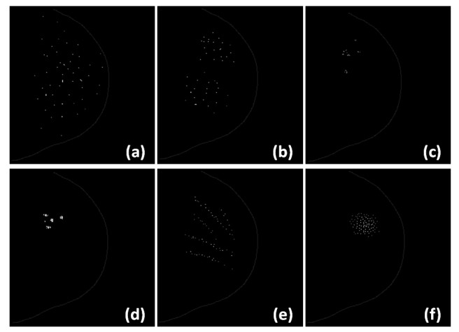
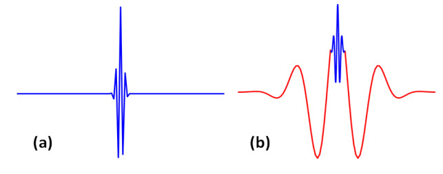
Figures(2)  /  Tables(2)

/

DownLoad:  Full-Size Img  PowerPoint
Return
Return

Catalog