Note on prescribed-time stability of impulsive piecewise-smooth differential systems and application in networks

Chenchen Li; Chunyan Zhang; Lichao Feng; Zhihui Wu; Chenchen Li; Chunyan Zhang; Lichao Feng; Zhihui Wu

doi:10.3934/nhm.2024043

Networks and Heterogeneous Media

2024, Volume 19, Issue 3: 970-991. doi: 10.3934/nhm.2024043

Previous Article Next Article

Research article

Note on prescribed-time stability of impulsive piecewise-smooth differential systems and application in networks

1.
College of Science, North China University of Science and Technology, Tangshan 063210, China
2.
School of Automation, Harbin University of Science and Technology, Harbin 150080, China

Received: 13 July 2024 Revised: 26 August 2024 Accepted: 13 September 2024 Published: 24 September 2024

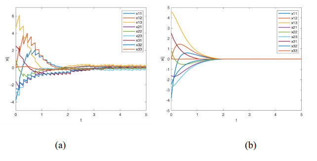
We explored the prescribed-time stability (PTSt) of impulsive piecewise smooth differential systems (IPSDS) based on the Lyapunov theory and set-valued analysis technology, allowing flexibility in selecting the settling time as desired. Furthermore, by developing a feedback controller, we employed the theoretical results to evaluate the synchronization behavior of impulsive piecewise-smooth network systems (IPSNS) within a prescribed time frame and obtained novel criteria to guarantee the synchronization objective. A numerical example was presented to validate the accuracy of the results.
- feedback controller,
- impulsive piecewise-smooth differential systems,
- prescribed-time stability,
- prescribed-time synchronization
Citation: Chenchen Li, Chunyan Zhang, Lichao Feng, Zhihui Wu. Note on prescribed-time stability of impulsive piecewise-smooth differential systems and application in networks[J]. Networks and Heterogeneous Media, 2024, 19(3): 970-991. doi: 10.3934/nhm.2024043

Related Papers:

Abstract

We explored the prescribed-time stability (PTSt) of impulsive piecewise smooth differential systems (IPSDS) based on the Lyapunov theory and set-valued analysis technology, allowing flexibility in selecting the settling time as desired. Furthermore, by developing a feedback controller, we employed the theoretical results to evaluate the synchronization behavior of impulsive piecewise-smooth network systems (IPSNS) within a prescribed time frame and obtained novel criteria to guarantee the synchronization objective. A numerical example was presented to validate the accuracy of the results.

References

[1]	R. W. Brockett, Asymptotic stability and feedback stabilization, Differ. Geom. Control Theory, 27 (1983), 181–191.
[2]	S. P. Bhat, D. S. Bernstein, Finite-time stability of continuous autonomous systems, SIAM J. Control Optim., 38 (2000), 751–766. https://doi.org/10.1137/S0363012997321358 doi: 10.1137/S0363012997321358
[3]	W. M. Haddad, Q. Hui, Dissipativity theory for discontinuous dynamical systems: Basic input, state, and output properties, and finite-time stability of feedback interconnections, Nonlinear Anal.: Hybrid Syst., 3 (2009), 551–564. https://doi.org/10.1016/j.nahs.2009.04.006
[4]	A. Polyakov, Nonlinear feedback design for fixed-time stabilization of linear control systems, IEEE Trans. Autom. Control, 57 (2011), 2106–2110. https://doi.org/10.1109/TAC.2011.2179869 doi: 10.1109/TAC.2011.2179869
[5]	B. Zhou, Finite-time stability analysis and stabilization by bounded linear time-varying feedback, Automatica, 121 (2020), 109191. https://doi.org/10.1016/j.automatica.2020.109191 doi: 10.1016/j.automatica.2020.109191
[6]	F. C. Kong, Q. X. Zhu, T. W. Huang, New fixed-time stability lemmas and applications to the discontinuous fuzzy inertial neural networks, IEEE Trans. Fuzzy Syst., 29 (2020), 3711–3722. https://doi.org/10.1109/TFUZZ.2020.3026030 doi: 10.1109/TFUZZ.2020.3026030
[7]	J. Holloway, M. Krstic, Prescribed-time observers for linear systems in observer canonical form, IEEE Trans. Autom. Control, 64 (2019), 3905–3912. https://doi.org/10.1109/TAC.2018.2890751 doi: 10.1109/TAC.2018.2890751
[8]	B. Zhou, Y. Shi, Prescribed-time stabilization of a class of nonlinear systems by linear time-varying feedback, IEEE Trans. Autom. Control, 66 (2021), 6123–6130. https://doi.org/10.1109/TAC.2021.3061645 doi: 10.1109/TAC.2021.3061645
[9]	L. C. Feng, M. Y. Dai, N. Ji, Y. L. Zhang, L. P. Du, Prescribed-time stabilization of nonlinear systems with uncertainties/disturbances by improved time-varying feedback control, AIMS Math., 9 (2024), 23859–23877. https://doi.org/10.3934/math.20241159 doi: 10.3934/math.20241159
[10]	D. X. Cao, X. X. Zhou, X. Y. Guo, N. Song, Limit cycle oscillation and dynamical scenarios in piecewise-smooth nonlinear systems with two-sided constraints, Nonlinear Dyn., 112 (2024), 9887–9914. https://doi.org/10.1007/s11071-024-09589-6 doi: 10.1007/s11071-024-09589-6
[11]	M. R. Jeffrey, Smoothing tautologies, hidden dynamics, and sigmoid asymptotics for piecewise smooth systems, Chaos, 25 (2015), 103125. https://doi.org/10.1063/1.4934204 doi: 10.1063/1.4934204
[12]	B. Samadi, Stability Analysis and Controller Synthesis for A Class of Piecewise Smooth Systems, Ph.D thesis, Concordia University, 2008.
[13]	S. Chen, Z. D. Du, Stability and perturbations of homoclinic loops in a class of piecewise smooth systems, Int. J. Bifurcation Chaos, 25 (2015), 1550114. https://doi.org/10.1142/S021812741550114X doi: 10.1142/S021812741550114X
[14]	B. Samadi, L. Rodrigues, A unified dissipativity approach for stability analysis of piecewise smooth systems, Automatica, 47 (2011), 2735–2742. https://doi.org/10.1016/j.automatica.2011.09.018 doi: 10.1016/j.automatica.2011.09.018
[15]	P. Glendinning, M. R. Jeffrey, An Introduction to Piecewise Smooth Dynamics, Springer International Publishing, Switzerland, 2019. https://doi.org/10.1007/978-3-030-23689-2
[16]	X. N. Li, H. Q. Wu, J. D. Cao, Prescribed-time synchronization in networks of piecewise smooth systems via a nonlinear dynamic event-triggered control strategy, Math. Comput. Simul., 203 (2023), 647–668. https://doi.org/10.1016/j.matcom.2022.07.010 doi: 10.1016/j.matcom.2022.07.010
[17]	W. M. Haddad, V. Chellaboina, N. A. Kablar, Non-linear impulsive dynamical systems, Part I: Stability and dissipativity, Int. J. Control, 74 (2001), 1631–1658. https://doi.org/10.1080/00207170110081705 doi: 10.1080/00207170110081705
[18]	S. G. Nersesov, W. M. Haddad, Control vector Lyapunov functions for large-scale impulsive dynamical system, Nonlinear Anal. Hybrid Syst., 1 (2007), 223–243. https://doi.org/10.1016/j.nahs.2006.10.006 doi: 10.1016/j.nahs.2006.10.006
[19]	Q. Xi, Z. L. Liang, X. D. Li, Uniform finite-time stability of nonlinear impulsive time-varying systems, Appl. Math. Modell., 91 (2021), 913–922. https://doi.org/10.1016/j.apm.2020.10.002 doi: 10.1016/j.apm.2020.10.002
[20]	Q. Xi, X. Z. Liu, X. D. Li, Practical finite-time stability of nonlinear systems with delayed impulsive control, IEEE Trans. Syst. Man Cybern.: Syst., 53 (2023), 7317–7325. https://doi.org/10.1109/TSMC.2023.3296481 doi: 10.1109/TSMC.2023.3296481
[21]	S. W. Zhao, J. T. Sun, L. Liu, Finite-time stability of linear time-varying singular systems with impulsive effects, Int. J. Control, 81 (2008), 1824–1829. https://doi.org/10.1080/00207170801898893 doi: 10.1080/00207170801898893
[22]	M. A. Jamal, R. Kumar, S. Mukhopadhyay, S. Das, Fixed-time stability of dynamical systems with impulsive effects, J. Franklin Inst., 359 (2022), 3164–3182. https://doi.org/10.1016/j.jfranklin.2022.02.016 doi: 10.1016/j.jfranklin.2022.02.016
[23]	Q. H. Wang, A. Abdurahman, Fixed-time stability analysis of general impulsive systems and application to synchronization of complex networks with hybrid impulses, Neurocomputing, 601 (2024), 128218. https://doi.org/10.1016/j.neucom.2024.128218 doi: 10.1016/j.neucom.2024.128218
[24]	H. F. Li, C. D. Li, T. W. Huang, D. Q. Ouyang, Fixed-time stability and stabilization of impulsive dynamical systems, J. Franklin Inst., 354 (2017), 8626–8644. https://doi.org/10.1016/j.jfranklin.2017.09.036 doi: 10.1016/j.jfranklin.2017.09.036
[25]	X. Y. He, X. D. Li, S. J. Song, Prescribed-time stabilization of nonlinear systems via impulsive regulation, IEEE Trans. Syst. Man Cybern.: Syst., 53 (2022), 981–985. https://doi.org/10.1109/TSMC.2022.3188874 doi: 10.1109/TSMC.2022.3188874
[26]	X. N. Li, H. Q. Wu, J. D. Cao, A new prescribed-time stability theorem for impulsive piecewise-smooth systems and its application to synchronization in networks, Appl. Math. Modell., 115 (2023), 385–397. https://doi.org/10.1016/j.apm.2022.10.051 doi: 10.1016/j.apm.2022.10.051
[27]	M. Coraggio, P. De Lellis, M. di Bernardo, Convergence and synchronization in networks of piecewise-smooth systems via distributed discontinuous coupling, Automatica, 129 (2021), 109596. https://doi.org/10.1016/j.automatica.2021.109596 doi: 10.1016/j.automatica.2021.109596
[28]	L. Dieci, C. Elia, Master stability function for piecewise smooth Filippov networks, Automatica, 152 (2023), 110939. https://doi.org/10.1016/j.automatica.2023.110939 doi: 10.1016/j.automatica.2023.110939
[29]	J. Chen, X. R. Li, X. Q. Wu, G. B. Shen, Prescribed-time synchronization of complex dynamical networks with and without time-varying delays, IEEE Trans. Network Sci. Eng., 9 (2022), 4017–4027. https://doi.org/10.1109/TNSE.2022.3191348 doi: 10.1109/TNSE.2022.3191348
[30]	L. L. Xu, X. W. Liu, Prescribed-time synchronization of multiweighted and directed complex networks, IEEE Trans. Autom. Control, 68 (2023), 8208–8215. https://doi.org/10.1109/TAC.2023.3292148 doi: 10.1109/TAC.2023.3292148
[31]	J. R. Yang, G. C. Chen, S. Zhu, S. P. Wen, J. H. Hu, Fixed/prescribed-time synchronization of BAM memristive neural networks with time-varying delays via convex analysis, Neural Networks, 163 (2023), 53–63. https://doi.org/10.1016/j.neunet.2023.03.031 doi: 10.1016/j.neunet.2023.03.031
[32]	Q. Tang, S. C. Qu, C. Zhang, Z. W. Tu, Y. T. Cao, Effects of impulse on prescribed-time synchronization of switching complex networks, Neural Networks, 174 (2024), 106248. https://doi.org/10.1016/j.neunet.2024.106248 doi: 10.1016/j.neunet.2024.106248
[33]	F. V. Difonzo, Isochronous attainable manifolds for piecewise smooth dynamical systems, Qual. Theory Dyn. Syst., 21 (2022), 6. https://doi.org/10.1007/s12346-021-00536-z doi: 10.1007/s12346-021-00536-z
[34]	A. F. Filippov, Differential Equations with Discontinuous Righthand Sides: Control Systems, Springer Science & Business Media, Berlin, 2013. https://doi.org/10.1007/978-94-015-7793-9
[35]	J. Cortes, Discontinuous dynamical systems, IEEE Control Syst. Mag., 28 (2008), 36–73. https://doi.org/10.1109/MCS.2008.919306 doi: 10.1109/MCS.2008.919306
[36]	Y. D. Song, Y. J. Wang, J. Holloway, M. Krstic, Time-varying feedback for regulation of normal-form nonlinear systems in prescribed finite time, Automatica, 83 (2017), 243–251. https://doi.org/10.1016/j.automatica.2017.06.008 doi: 10.1016/j.automatica.2017.06.008
[37]	A. Bacciotti, F. Ceragioli, Stability and stabilization of discontinuous systems and nonsmooth Lyapunov functions, ESAIM. Control. Optim. Calc. Var., 4 (1999), 361–376. https://doi.org/10.1051/cocv:1999113 doi: 10.1051/cocv:1999113
[38]	Y. J. Shen, X. H. Xia, Semi-global finite-time observers for nonlinear systems, Automatica, 44 (2008), 3152–3156. https://doi.org/10.1016/j.automatica.2008.05.015 doi: 10.1016/j.automatica.2008.05.015
[39]	Y. J. Shen, Y. H. Huang, Uniformly observable and globally Lipschitzian nonlinear systems admit global finite-time observers, IEEE Trans. Autom. Control, 54 (2009), 2621–2625. https://doi.org/10.1109/TAC.2009.2029298 doi: 10.1109/TAC.2009.2029298
[40]	P. J. Ning, C. C. Hua, K. Li, H. Li, A novel theorem for prescribed-time control of nonlinear uncertain time-delay systems, Automatica, 152 (2023), 111009. https://doi.org/10.1016/j.automatica.2023.111009 doi: 10.1016/j.automatica.2023.111009
[41]	L. C. Feng, L. Liu, J. D. Cao, L. Rutkowski, G. P. Lu, General decay stability for nonautonomous neutral stochastic systems with time-varying delays and Markovian switching, IEEE Trans. Cybern., 52 (2022): 5441–5453. https://doi.org/10.1109/TCYB.2020.3031992 doi: 10.1109/TCYB.2020.3031992
[42]	D. Chalishajar, D. Kasinathan, R. Kasinathan, R. Kasinathan, Exponential stability, T-controllability and optimal controllability of higher-order fractional neutral stochastic differential equation via integral contractor, Chaos, Solitons Fractals, 186 (2024), 115278. https://doi.org/10.1016/j.chaos.2024.115278 doi: 10.1016/j.chaos.2024.115278
[43]	D. Chalishajar, R. Kasinathan, Kasinathan R, S. Varshini, On solvability and optimal controls for impulsive stochastic integrodifferential varying-coefficient model, Automatika, 65 (2024), 1271–1283. https://doi.org/10.1080/00051144.2024.2361212 doi: 10.1080/00051144.2024.2361212
[44]	D. Chalishajar, R. Kasinathan, R. Kasinathan, Existence and Stability Results for Time-Dependent Impulsive Neutral Stochastic Partial Integrodifferential Equations with Rosenblatt Process and Poisson Jumps, Tatra Mt. Math. Publ., 00 (2024), 1–24. https://doi.org/10.2478/tmmp-2024-0002 doi: 10.2478/tmmp-2024-0002

Reader Comments

Your name:*

Email:*
© 2024 the Author(s), licensee AIMS Press. This is an open access article distributed under the terms of the Creative Commons Attribution License (http://creativecommons.org/licenses/by/4.0)