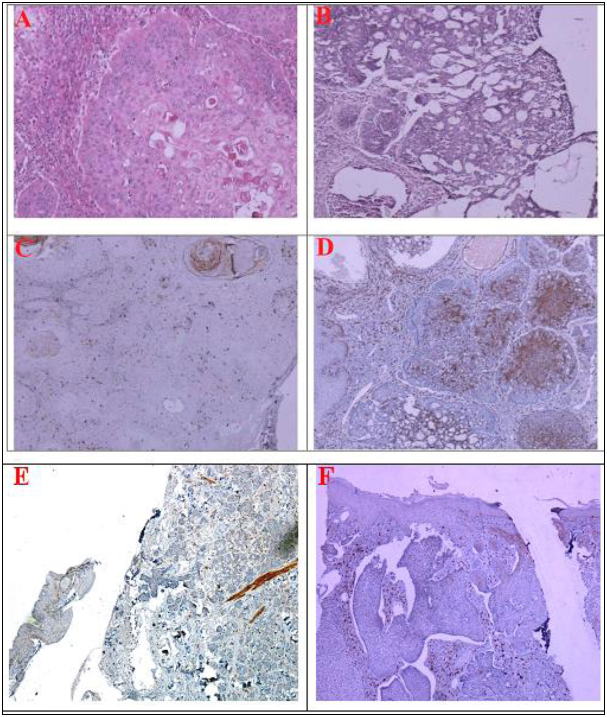
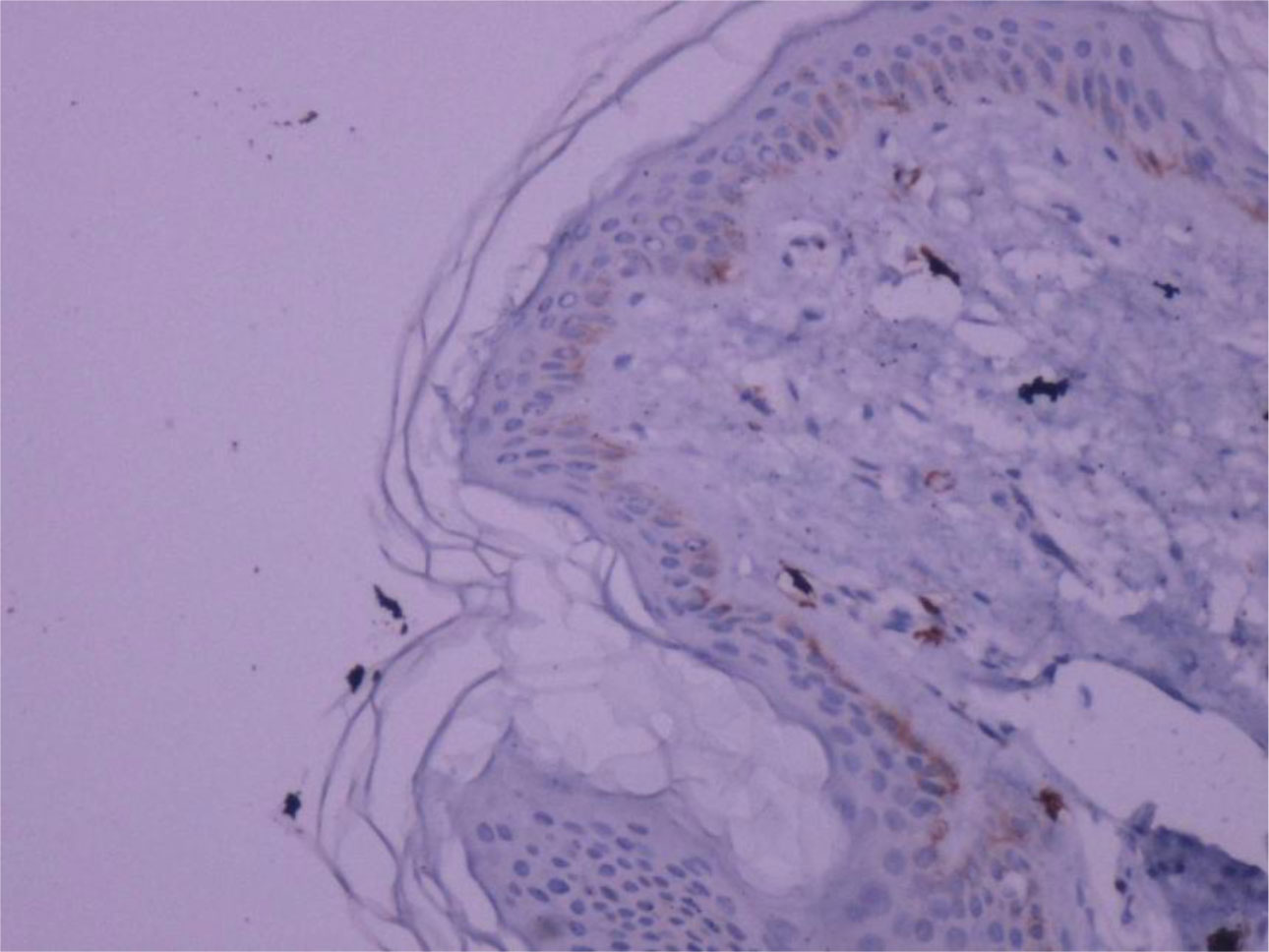
Squamous cell carcinoma (SCC) and Basal cell carcinoma (BCC) of the skin are the most common malignant tumors in humans. The c-Kit (CD117) is a tyrosine kinase receptor protein that affects the behavior of some tumors and can be a target for new treatments. This study was designed to determine the expression of CD117 in patients with SCC and BCC. In this retrospective study, 69 paraffin blocks of specimens with a diagnosis of SCC and BCC from limbs, head/neck, trunk, and unknown sites were selected. Tumor tissue samples of 40 SCC and 29 BCC cases were then analyzed by immunohistochemistry. The monoclonal CD117 antibody was used. The severity and extent of tumor staining were grouped as follows: negative; weakly positive; moderately positive; and strongly positive. The CD117 was detected positive in 26 (89.7%) BCCs and only in 5 (12.5%) of SCCs. We detected a significant difference between the expression of CD117 in patients with SCC and BCC (P < 0.05). No significant relationship was shown between the marker expression and the lesion site in patients with SCC or BCC (P > 0.05). On the contrary, a significant relationship between CD117 expression and histopathologic grading was identified in patients with SCC (P < 0.05). According to our results, the expression of CD117 is significantly increased in BCCs than SCCs and this may be of benefit for diagnostic purposes in challenging cases and also for therapeutic purposes including targeted therapy if indicated.
Citation: Mazaher Ramezani, Marziyeh Masnadjam, Ali Azizi, Elisa Zavattaro, Sedigheh Khazaei, Masoud Sadeghi. Evaluation of c-Kit (CD117) expression in patients with squamous cell carcinoma (SCC) and basal cell carcinoma (BCC) of the skin[J]. AIMS Molecular Science, 2021, 8(1): 51-59. doi: 10.3934/molsci.2021004
Squamous cell carcinoma (SCC) and Basal cell carcinoma (BCC) of the skin are the most common malignant tumors in humans. The c-Kit (CD117) is a tyrosine kinase receptor protein that affects the behavior of some tumors and can be a target for new treatments. This study was designed to determine the expression of CD117 in patients with SCC and BCC. In this retrospective study, 69 paraffin blocks of specimens with a diagnosis of SCC and BCC from limbs, head/neck, trunk, and unknown sites were selected. Tumor tissue samples of 40 SCC and 29 BCC cases were then analyzed by immunohistochemistry. The monoclonal CD117 antibody was used. The severity and extent of tumor staining were grouped as follows: negative; weakly positive; moderately positive; and strongly positive. The CD117 was detected positive in 26 (89.7%) BCCs and only in 5 (12.5%) of SCCs. We detected a significant difference between the expression of CD117 in patients with SCC and BCC (P < 0.05). No significant relationship was shown between the marker expression and the lesion site in patients with SCC or BCC (P > 0.05). On the contrary, a significant relationship between CD117 expression and histopathologic grading was identified in patients with SCC (P < 0.05). According to our results, the expression of CD117 is significantly increased in BCCs than SCCs and this may be of benefit for diagnostic purposes in challenging cases and also for therapeutic purposes including targeted therapy if indicated.

| [1] |
Perry DM, Barton V, Alberg AJ (2017) Epidemiology of Keratinocyte Carcinoma. Curr Dermatol Rep 6: 161-168. doi: 10.1007/s13671-017-0185-6

|
| [2] |
Subramaniam P, Olsen CM, Thompson BS, et al. (2017) Anatomical distributions of basal cell carcinoma and squamous cell carcinoma in a population-based study in Queensland, Australia. JAMA Dermatol 153: 175-182. doi: 10.1001/jamadermatol.2016.4070
|
| [3] |
Karia PS, Han J, Schmults CD (2013) Cutaneous squamous cell carcinoma: estimated incidence of disease, nodal metastasis, and deaths from the disease in the United States, 2012. J Am Acad Dermatol 68: 957-966. doi: 10.1016/j.jaad.2012.11.037
|
| [4] |
Liang J, Wu YL, Chen BJ, et al. (2013) The C-Kit Receptor-Mediated Signal Transduction and Tumor-Related Diseases. Int J Biol Sci 9: 435-443. doi: 10.7150/ijbs.6087
|
| [5] | Jalayer Naderi N, Ashouri M, Tirgari F, et al. (2011) An immunohistochemical study of CD117 Ckit in adenoid cystic carcinoma and polymorphouse low grade adenocarcinoma salivary gland tumors. SRJSU 90: 1-9. |
| [6] |
Went PT, Dirnhofer S, Bundi M, et al. (2004) Prevalence of KIT expression in human tumors. J Clin Oncol 22: 4514-4522. doi: 10.1200/JCO.2004.10.125
|
| [7] | Matsuda R, Takahashi T, Nakamura S, et al. (1993) Expression of the c-kit protein in human solid tumors and in corresponding fetal and adult normal tissues. Am J Pathol 142: 339-346. |
| [8] |
Terada T (2013) Expression of NCAM (CD56), chromogranin A, synaptophysin, c-KIT (CD117) and PDGFRA in normal non-neoplastic skin and basal cell carcinoma: an immunohistochemical study of 66 consecutive cases. Med Oncol 30: 444. doi: 10.1007/s12032-012-0444-0
|
| [9] | Leon A, Ceauşu ZE, Ceauşu M, et al. (2009) Mast cells and dendritic cells in basal cell carcinoma. Rom J Morphol Embryol 50: 85-90. |
| [10] |
Dessauvagie BF, Wood BA (2015) CD117 and CD43 are useful adjuncts in the distinction of adenoid cystic carcinoma from adenoid basal cell carcinoma. Pathology 47: 130-133. doi: 10.1097/PAT.0000000000000209
|
| [11] |
Yang DT, Holden JA, Florell SR (2004) CD117, CK20, TTF-1, and DNA topoisomerase II-alpha antigen expression in small cell tumors. J Cutan Pathol 31: 254-261. doi: 10.1111/j.0303-6987.2003.00175.x
|
| [12] |
Castillo JM, Knol AC, Nguyen JM, et al. (2016) Immunohistochemical markers of advanced basal cell carcinoma: CD56 is associated with a lack of response to vismodegib. Eur J Dermatol 26: 452-459. doi: 10.1684/ejd.2016.2826
|
| [13] |
Pelosi G, Barisella M, Pasini F, et al. (2004) CD117 immunoreactivity in stage I adenocarcinoma and squamous cell carcinoma of the lung: relevance to prognosis in a subset of adenocarcinoma patients. Mod Pathol 17: 711-721. doi: 10.1038/modpathol.3800110
|
| [14] |
Kriegsmann M, Muley T, Harms A, et al. (2015) Differential diagnostic value of CD5 and CD117 expression in thoracic tumors: A large scale study of 1465 non-small cell lung cancer cases. Diagn Pathol 10: 210. doi: 10.1186/s13000-015-0441-7
|
| [15] |
Nakagawa K, Matsuno Y, Kunitoh H, et al. (2005) Immunohistochemical KIT (CD117) expression in thymic epithelial tumors. Chest 128: 140-144. doi: 10.1378/chest.128.1.140
|
| [16] |
Goto K, Takai T, Fukumoto T, et al. (2016) CD117 (KIT) is a useful immunohistochemical marker for differentiating porocarcinoma from squamous cell carcinoma. J Cutan Pathol 43: 219-226. doi: 10.1111/cup.12632
|
| [17] |
Goto K (2015) Immunohistochemistry for CD117 (KIT) is effective in distinguishing cutaneous adnexal tumors with apocrine/eccrine or sebaceous differentiation from other epithelial tumors of the skin. J Cutan Pathol 42: 480-488. doi: 10.1111/cup.12492
|
| [18] |
Andreadis D, Epivatianos A, Poulopoulos A, et al. (2006) Detection of C-KIT (CD117) molecule in benign and malignant salivary gland tumours. Oral Oncol 42: 56-64. doi: 10.1016/j.oraloncology.2005.06.014
|
| [19] |
Penner CR, Folpe AL, Budnick SD (2002) C-kit expression distinguishes salivary gland adenoid cystic carcinoma from polymorphous low-grade adenocarcinoma. Mod Pathol 15: 687-691. doi: 10.1097/01.MP.0000018973.17736.F8
|
| [20] |
Edwards PC, Bhuiya T, Kelsch RD (2003) C-kit expression in the salivary gland neoplasms adenoid cystic carcinoma, polymorphous low-grade adenocarcinoma, and monomorphic adenoma. Oral Surg Oral Med Oral Pathol Oral Radiol Endod 95: 586-593. doi: 10.1067/moe.2003.31
|
| [21] |
Atef A, El-Rashidy MA, Abdel Azeem A, et al. (2019) The Role of Stem Cell Factor in Hyperpigmented Skin Lesions. Asian Pac J Cancer Prev 20: 3723-3728. doi: 10.31557/APJCP.2019.20.12.3723
|
| [22] |
Zilberg C, Lee MW, Kraitsek S, et al. (2020) Is high-risk cutaneous squamous cell carcinoma of the head and neck a suitable candidate for current targeted therapies? J Clin Pathol 73: 17-22. doi: 10.1136/jclinpath-2019-206038
|
Figures(2) / Tables(2)

Mazaher Ramezani, Marziyeh Masnadjam, Ali Azizi, Elisa Zavattaro, Sedigheh Khazaei, Masoud Sadeghi. Evaluation of c-Kit (CD117) expression in patients with squamous cell carcinoma (SCC) and basal cell carcinoma (BCC) of the skin[J]. AIMS Molecular Science, 2021, 8(1): 51-59. doi: 10.3934/molsci.2021004


 DownLoad: