Diversity of ligninolytic ascomycete fungi associated with the bleached leaf litter in subtropical and temperate forests

Momoka Yoneda; Hiroki Ameno; Ayaka Nishimura; Kohei Tabuchi; Yuki Hatano; Takashi Osono; Momoka Yoneda; Hiroki Ameno; Ayaka Nishimura; Kohei Tabuchi; Yuki Hatano; Takashi Osono

doi:10.3934/microbiol.2024042

AIMS Microbiology

2024, Volume 10, Issue 4: 973-985. doi: 10.3934/microbiol.2024042

Previous Article Next Article

Research article

Diversity of ligninolytic ascomycete fungi associated with the bleached leaf litter in subtropical and temperate forests

1.
Graduate School of Science and Engineering, Doshisha University, Kyotanabe, Kyoto 610-0394, Japan
2.
Faculty of Science and Engineering, Doshisha University, Kyotanabe, Kyoto 610-0394, Japan

Received: 14 June 2024 Revised: 01 November 2024 Accepted: 12 November 2024 Published: 15 November 2024

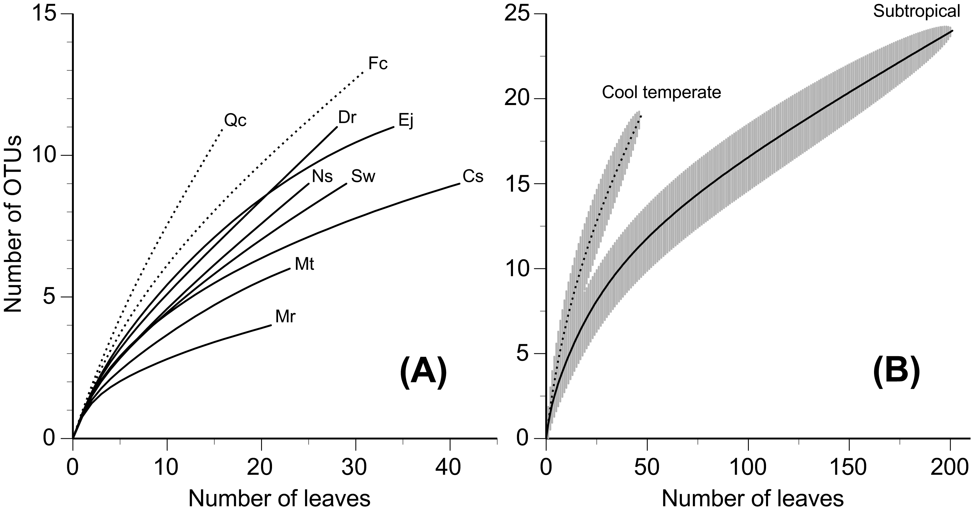
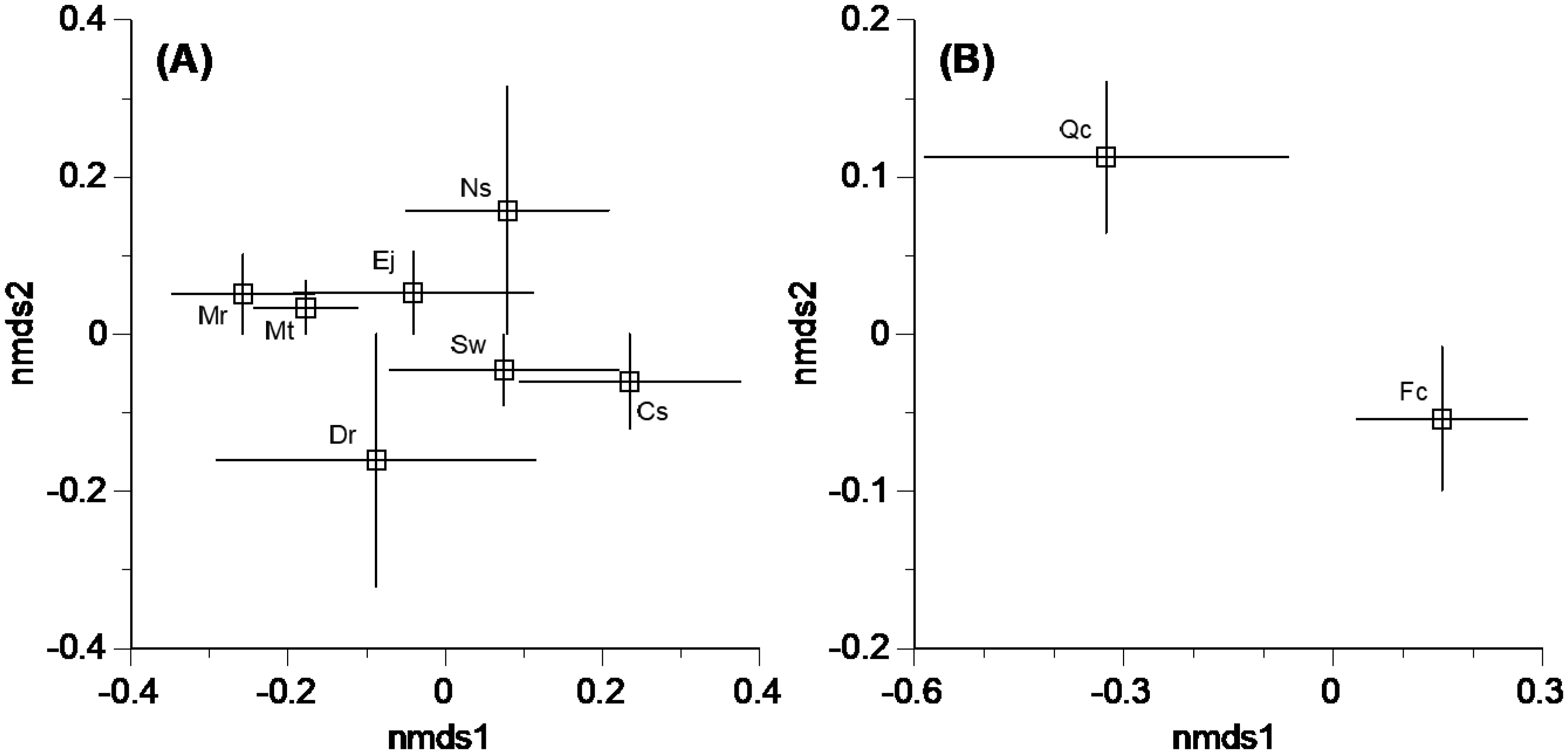
Little is known regarding the diversity patterns of Xylariaceae and Hypoxylaceae (Ascomycota) fungi taking part in the lignin decomposition of leaf litter from different tree species and under different climatic regions. The alpha and beta diversity of Xylariaceae and Hypoxylaceae fungi was investigated on bleached leaf litter from nine subtropical and cool temperate tree species in Japan. A total of 248 fungal isolates, obtained from 480 leaves from the nine tree species, were classified into 43 operational taxonomic units (OTUs) with a 97% similarity threshold and were assigned to nine genera of Xylariaceae and Hypoxylaceae. There was no overlap of fungal OTUs between subtropical and cool temperate trees. The mean number of fungal OTUs was generally higher in subtropical than cool temperate trees, whereas rarefaction curves depicting the numbers of OTU with respect to the number of leaves from which fungi were isolated were less steep in subtropical trees than in cool temperate trees, reflecting the dominance of major OTUs in the subtropical trees and indicating a higher species richness in cool temperate regions. Nonmetric multidimensional scaling showed general overlaps of fungal OTU compositions among tree species in the respective climatic regions, and one-way permutational multivariate analysis of variance indicated that the OTU composition was not significantly different between the tree species. These results suggest a wide host range and some geographic and climatic structures of distribution of these ligninolytic fungi.
- Ascomycota,
- dead leaves,
- fungal richness,
- Hypoxylaceae,
- lignin decomposition,
- Xylariaceae
Citation: Momoka Yoneda, Hiroki Ameno, Ayaka Nishimura, Kohei Tabuchi, Yuki Hatano, Takashi Osono. Diversity of ligninolytic ascomycete fungi associated with the bleached leaf litter in subtropical and temperate forests[J]. AIMS Microbiology, 2024, 10(4): 973-985. doi: 10.3934/microbiol.2024042

Related Papers:

Abstract

Little is known regarding the diversity patterns of Xylariaceae and Hypoxylaceae (Ascomycota) fungi taking part in the lignin decomposition of leaf litter from different tree species and under different climatic regions. The alpha and beta diversity of Xylariaceae and Hypoxylaceae fungi was investigated on bleached leaf litter from nine subtropical and cool temperate tree species in Japan. A total of 248 fungal isolates, obtained from 480 leaves from the nine tree species, were classified into 43 operational taxonomic units (OTUs) with a 97% similarity threshold and were assigned to nine genera of Xylariaceae and Hypoxylaceae. There was no overlap of fungal OTUs between subtropical and cool temperate trees. The mean number of fungal OTUs was generally higher in subtropical than cool temperate trees, whereas rarefaction curves depicting the numbers of OTU with respect to the number of leaves from which fungi were isolated were less steep in subtropical trees than in cool temperate trees, reflecting the dominance of major OTUs in the subtropical trees and indicating a higher species richness in cool temperate regions. Nonmetric multidimensional scaling showed general overlaps of fungal OTU compositions among tree species in the respective climatic regions, and one-way permutational multivariate analysis of variance indicated that the OTU composition was not significantly different between the tree species. These results suggest a wide host range and some geographic and climatic structures of distribution of these ligninolytic fungi.

Acknowledgments

We thank the staff at the Yona Experimental Forest of the University of the Ryukyus and the Sugadaira Montane Research Center of the University of Tsukuba for providing permission for field sampling; Dr. S. Matsuoka and Mr. Y. Nagata for help with fieldwork and laboratory work; Professor Dr. M. Hasegawa and Professor Dr. H. Tsutsumi for useful discussions; and Dr. E. Nakajima for critical reading of the manuscript. This work was supported by the Ministry of Education, Culture, Sports, Science, and Technology of Japan [No. 18K05731].

Conflict of interest

The authors declare no conflict of interest.

Author contributions

Conceptualization: TO; Sample collection: KT, YH, TO; Fungal isolation: MY, HA, AN; Molecular analysis: MY, HA, AN, YH; Data analysis: MY, YH, TO; Original draft preparation: MY, TO; Writing – review and editing: MY, YH, TO; Funding acquisition: TO.

References

[1]	Baldrian P (2017) Forest microbiome: Diversity, complexity and dynamics. FEMS Microbiol Rev 41: 109-130. https://doi.org/10.1093/femsre/fuw040
[2]	Eriksson KE, Blanchette RA, Ander P (1990) Microbial and enzymatic degradation of wood and wood components. New York: Springer. https://doi.org/10.1007/978-3-642-46687-8
[3]	Van der Wal A, Geydan TD, Kuype TW, et al. (2013) A thready affair: Linking fungal diversity and community dynamics to terrestrial decomposition processes. FEMS Microbiol Rev 37: 477-494. https://doi.org/10.1111/1574-6976.12001
[4]	Miyamoto T, Koda K, Kawaguchi A, et al. (2017) Ligninolytic activity at 0 °C of fungi on oak leaves under snow cover in a mixed forest in Japan. Microb Ecol 74: 322-331. https://doi.org/10.1007/s00248-017-0952-8
[5]	Fukasawa Y (2021) Ecological impacts of fungal wood decay types: A review of current knowledge and future research directions. Ecol Res 36: 910-931. https://doi.org/10.1111/1440-1703.12260
[6]	Boddy L, Frankland JC, van West P (2008) Ecology of Saprotrophic Basidiomycetes. London: Elsevier.
[7]	Whalley AJS (1996) The xylariaceous way of life. Mycol Res 100: 897-922. https://doi.org/10.1016/S0953-7562(96)80042-6
[8]	Rogers JD (2000) Thoughts and musings on tropical Xylariaceae. Mycol Res 104: 1412-1420. https://doi.org/10.1017/S0953756200003464
[9]	Osono T, Matsuoka S, Hirose D (2021) Diversity and host recurrence of fungi associated with the bleached leaf litter in a subtropical forest. Fungal Ecol 54: 101-113. https://doi.org/10.1016/j.funeco.2021.101113
[10]	Osono T, Tateno O, Masuya H (2013) Diversity and ubiquity of xylariaceous endophytes in live and dead leaves of temperate forest trees. Mycoscience 54: 54-61. https://doi.org/10.1016/j.myc.2012.08.003
[11]	Enoki T (2003) Microtopography and distribution of canopy trees in a subtropical evergreen broad-leaved forest in the northern part of Okinawa Island, Japan. Ecol Res 18: 103-113. https://doi.org/10.1046/j.1440-1703.2003.00549.x
[12]	Osono T, Ishii Y, Hirose D (2008) Fungal colonization and decomposition of Castanopsis sieboldii leaf litter in a subtropical forest. Ecol Res 23: 909-917. https://doi.org/10.1007/s11284-007-0455-z
[13]	Tanabe AS, Toju H (2013) Two new computational methods for universal DNA barcoding: a benchmark using barcode sequences of bacteria, archaea, animals, fungi, and land plants. PloS One 8: e76910. https://doi.org/10.1371/journal.pone.0076910
[14]	Camacho C, Coulouris G, Avagyan V, et al. (2009) BLAST+: architecture and applications. BMC Bioinformatics 10: 421. https://doi.org/10.1186/1471-2105-10-421
[15]	Oksanen J, Simpson GL Package ‘vegan’ Version 2.6-4 (2022). Avaliable at: http://cran.r-project.org/web/packages/vegan/index.html. (accessed February 29, 2024)
[16]	Nilsson T, Daniel G (1989) Chemistry and microscopy of wood decay by some higher ascomycetes. Holzforschung 43: 11-18. https://doi.org/10.1515/hfsg.1989.43.1.11
[17]	Pointing SB, Pelling AL, Smith GJD, et al. (2005) Screening of basidiomycetes and xylariaceous fungi for lignin peroxidase and laccase gene-specific sequences. Mycol Res 109: 115-124. https://doi.org/10.1017/S0953756204001376
[18]	Osono T (2020) Decomposition of organic chemical components in wood by tropical Xylaria species. J Fungi 6: 186. https://doi.org/10.3390/jof6040186
[19]	Wendt L, Sir EB, Kuhnert E, et al. (2018) Resurrection and emendation of the Hypoxylaceae, recognised from a multigene phylogeny of the Xylariales. Mycol Prog 17: 115-154. https://doi.org/10.1007/s11557-017-1311-3
[20]	Hyde KD, de Silva NI, Jeewon R, et al. (2020) AJOM new records and collections of fungi: 1-100. Asian J Mycol 3: 22-294. https://doi.org/10.5943/ajom/3/1/3
[21]	Franco MEE, Wisecaver JH, Arnold AE, et al. (2022) Ecological generalism drives hyperdiversity of secondary metabolite gene clusters in xylarialean endophytes. New Phytol 233: 1317-1330. https://doi.org/10.1111/nph.17873
[22]	Ikeda A, Matsuoka S, Masuya H, et al. (2014) Comparison of the diversity, composition, and host recurrence of xylariaceous endophytes in subtropical, cool temperate, and subboreal regions in Japan. Popul Ecol 56: 289-300. https://doi.org/10.1007/s10144-013-0412-3
[23]	Zhou D, Hyde KD (2001) Host-specificity, host-exclusivity, and host recurrence in saprobic fungi. Mycol Res 105: 1449-1457. https://doi.org/10.1017/S0953756201004713
[24]	Læssøe T, Lodge DJ (1994) Three host-specific Xylaria species. Mycologia 86: 436-446. https://doi.org/10.1080/00275514.1994.12026431
[25]	Petrini O, Petrini LE, Rodrigues KF (1995) Xylariaceous endophytes: an exercise in biodiversity. Fitopatol Bras 20: 531-539.
[26]	Okane I, Srikitikulchai P, Tabuchi Y, et al. (2012) Recognition and characterization of four Thai xylariaceous fungi inhabiting various tropical foliages as endophytes by DNA sequences and host plant preference. Mycoscience 53: 122-132. https://doi.org/10.1007/S10267-011-0149-9
[27]	Nilsson RH, Kristiansson E, Ryberg M, et al. (2008) Intraspecific ITS variability in the kingdom Fungi as expressed in the international sequence databases and its implications for molecular species identification. Evol Bioinform online 4: 193-201. https://doi.org/10.4137/EBO.S653
[28]	Liers C, Arnstadt T, Ullrich R, et al. (2011) Patterns of lignin degradation and oxidative enzyme secretion by different wood- and litter-colonizing basidiomycetes and ascomycetes grown on beech-wood. FEMS Microbiol Ecol 78: 91-102. https://doi.org/10.1111/j.1574-6941.2011.01144.x
[29]	Tabuchi K, Hirose D, Hasegawa M, et al. (2022) Metabolic diversity of xylariaceous fungi associated with leaf litter decomposition. J Fungi 8: 701. https://doi.org/10.3390/jof8070701

microbiol-10-04-042-s001.xlsx

Reader Comments

Your name:*

Email:*
© 2024 the Author(s), licensee AIMS Press. This is an open access article distributed under the terms of the Creative Commons Attribution License (http://creativecommons.org/licenses/by/4.0)