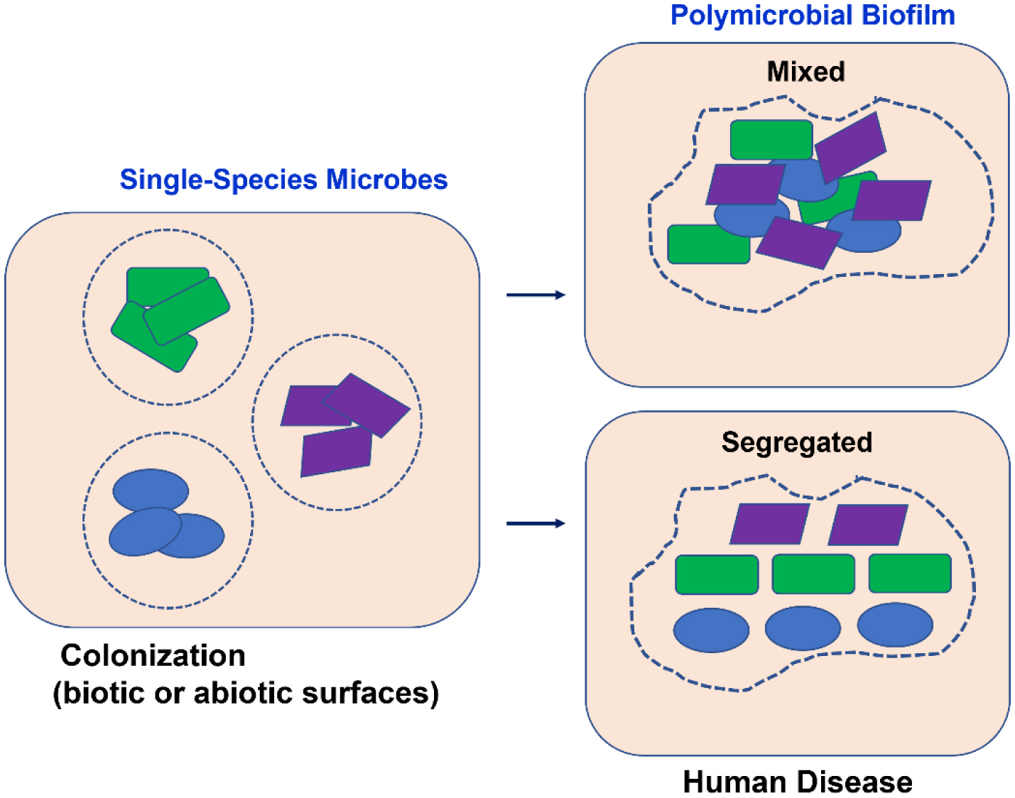
This review addresses the topic of biofilms, including their development and the interaction between different counterparts. There is evidence that various diseases, such as cystic fibrosis, otitis media, diabetic foot wound infections, and certain cancers, are promoted and aggravated by the presence of polymicrobial biofilms. Biofilms are composed by heterogeneous communities of microorganisms protected by a matrix of polysaccharides. The different types of interactions between microorganisms gives rise to an increased resistance to antimicrobials and to the host's defense mechanisms, with the consequent worsening of disease symptoms. Therefore, infections caused by polymicrobial biofilms affecting different human organs and systems will be discussed, as well as the role of the interactions between the gram-negative bacteria Pseudomonas aeruginosa, which is at the base of major polymicrobial infections, and other bacteria, fungi, and viruses in the establishment of human infections and diseases. Considering that polymicrobial biofilms are key to bacterial pathogenicity, it is fundamental to evaluate which microbes are involved in a certain disease to convey an appropriate and efficacious antimicrobial therapy.
Citation: Manuela Oliveira, Eva Cunha, Luís Tavares, Isa Serrano. P. aeruginosa interactions with other microbes in biofilms during co-infection[J]. AIMS Microbiology, 2023, 9(4): 612-646. doi: 10.3934/microbiol.2023032
This review addresses the topic of biofilms, including their development and the interaction between different counterparts. There is evidence that various diseases, such as cystic fibrosis, otitis media, diabetic foot wound infections, and certain cancers, are promoted and aggravated by the presence of polymicrobial biofilms. Biofilms are composed by heterogeneous communities of microorganisms protected by a matrix of polysaccharides. The different types of interactions between microorganisms gives rise to an increased resistance to antimicrobials and to the host's defense mechanisms, with the consequent worsening of disease symptoms. Therefore, infections caused by polymicrobial biofilms affecting different human organs and systems will be discussed, as well as the role of the interactions between the gram-negative bacteria Pseudomonas aeruginosa, which is at the base of major polymicrobial infections, and other bacteria, fungi, and viruses in the establishment of human infections and diseases. Considering that polymicrobial biofilms are key to bacterial pathogenicity, it is fundamental to evaluate which microbes are involved in a certain disease to convey an appropriate and efficacious antimicrobial therapy.

| [1] |
Pouget C, Dunyach-Remy C, Pantel A, et al. (2020) Biofilms in diabetic foot ulcers: Significance and clinical relevance. Microorganisms 8. https://doi.org/10.3390/microorganisms8101580 
|
| [2] |
Costerton JW, Stewart PS, Greenberg EP (1999) Bacterial biofilms: A common cause of persistent infections. Science 284: 1318-1322. https://doi.org/10.1126/science.284.5418.1318
|
| [3] |
Lam JS, MacDonald LA, Lam MY, et al. (1987) Production and characterization of monoclonal antibodies against serotype strains of Pseudomonas aeruginosa. Infect Immun 55: 1051-1057. https://doi.org/10.1128/iai.55.5.1051-1057.1987
|
| [4] |
Leid JG, Willson CJ, Shirtliff ME, et al. (2005) The exopolysaccharide alginate protects Pseudomonas aeruginosa biofilm bacteria from IFN-γ-mediated macrophage killing1. J Immunol 175: 7512-7518. https://doi.org/10.4049/jimmunol.175.11.7512
|
| [5] |
Wolcott R, Costerton JW, Raoult D, et al. (2013) The polymicrobial nature of biofilm infection. Clin Microbiol Infect 19: 107-112. https://doi.org/10.1111/j.1469-0691.2012.04001.x
|
| [6] |
Bjarnsholt T (2013) The role of bacterial biofilms in chronic infections. APMIS Suppl : 1-51. https://doi.org/10.1111/apm.12099
|
| [7] |
Brogden KA, Guthmiller JM, Taylor CE (2005) Human polymicrobial infections. Lancet 365: 253-255. https://doi.org/10.1016/s0140-6736(05)17745-9
|
| [8] |
Larsen MK, Thomsen TR, Moser C, et al. (2008) Use of cultivation-dependent and -independent techniques to assess contamination of central venous catheters: a pilot study. BMC Clin Pathol 8: 10. https://doi.org/10.1186/1472-6890-8-10
|
| [9] | Kumar A, Seenivasan MK, Inbarajan A (2021) A literature review on biofilm formation on silicone and poymethyl methacrylate used for maxillofacial prostheses. Cureus 13: e20029. https://doi.org/10.7759/cureus.20029 |
| [10] |
Rohacek M, Weisser M, Kobza R, et al. (2010) Bacterial colonization and infection of electrophysiological cardiac devices detected with sonication and swab culture. Circulation 121: 1691-1697. https://doi.org/10.1161/circulationaha.109.906461
|
| [11] |
Peters BM, Jabra-Rizk MA, O'May GA, et al. (2012) Polymicrobial interactions: impact on pathogenesis and human disease. Clin Microbiol Rev 25: 193-213. https://doi.org/10.1128/cmr.00013-11
|
| [12] |
Percival SL, McCarty SM, Lipsky B (2015) Biofilms and wounds: An overview of the evidence. Adv Wound Care New Rochelle 4: 373-381. https://doi.org/10.1089/wound.2014.0557
|
| [13] |
Beaudoin T, Yau YCW, Stapleton PJ, et al. (2017) Staphylococcus aureus interaction with Pseudomonas aeruginosa biofilm enhances tobramycin resistance. NPJ Biofilms Microbiomes 3: 25. https://doi.org/10.1038/s41522-017-0035-0
|
| [14] |
Windels EM, Michiels JE, Van den Bergh B, et al. (2019) Antibiotics: combatting tolerance to stop resistance. mBio 10. https://doi.org/10.1128/mbio.02095-19
|
| [15] |
Tay WH, Chong KK, Kline KA (2016) Polymicrobial-host interactions during infection. J Mol Biol 428: 3355-3371. https://doi.org/10.1016/j.jmb.2016.05.006
|
| [16] |
Wimmer MD, Friedrich MJ, Randau TM, et al. (2016) Polymicrobial infections reduce the cure rate in prosthetic joint infections: outcome analysis with two-stage exchange and follow-up ≥two years. Int Orthop 40: 1367-1373. https://doi.org/10.1007/s00264-015-2871-y
|
| [17] |
Dowd SE, Wolcott RD, Sun Y, et al. (2008) Polymicrobial nature of chronic diabetic foot ulcer biofilm infections determined using bacterial tag encoded FLX amplicon pyrosequencing (bTEFAP). PLoS One 3: e3326. https://doi.org/10.1371/journal.pone.0003326
|
| [18] |
Solano C, Echeverz M, Lasa I (2014) Biofilm dispersion and quorum sensing. Curr Opin Microbiol 18: 96-104. https://doi.org/10.1016/j.mib.2014.02.008
|
| [19] |
Hibbing ME, Fuqua C, Parsek MR, et al. (2010) Bacterial competition: surviving and thriving in the microbial jungle. Nat Rev Microbiol 8: 15-25. https://doi.org/10.1038/nrmicro2259
|
| [20] |
Smith H (1982) The role of microbial interactions in infectious disease. Philos Trans R Soc Lond B Biol Sci 297: 551-561. https://doi.org/10.1098/rstb.1982.0060
|
| [21] |
Hajishengallis G, Liang S, Payne MA, et al. (2011) Low-abundance biofilm species orchestrates inflammatory periodontal disease through the commensal microbiota and complement. Cell Host Microbe 10: 497-506. https://doi.org/10.1016/j.chom.2011.10.006
|
| [22] |
Korgaonkar A, Trivedi U, Rumbaugh KP, et al. (2013) Community surveillance enhances Pseudomonas aeruginosa virulence during polymicrobial infection. Proc Natl Acad Sci USA 110: 1059-1064. https://doi.org/10.1073/pnas.1214550110
|
| [23] |
Stacy A, McNally L, Darch SE, et al. (2016) The biogeography of polymicrobial infection. Nat Rev Microbiol 14: 93-105. https://doi.org/10.1038/nrmicro.2015.8
|
| [24] |
Simón-Soro A, Mira A (2015) Solving the etiology of dental caries. Trends Microbiol 23: 76-82. https://doi.org/10.1016/j.tim.2014.10.010
|
| [25] |
Yung DBY, Sircombe KJ, Pletzer D (2021) Friends or enemies? The complicated relationship between Pseudomonas aeruginosa and Staphylococcus aureus. Mol Microbiol 116: 1-15. https://doi.org/10.1111/mmi.14699
|
| [26] |
DeLeon S, Clinton A, Fowler H, et al. (2014) Synergistic interactions of Pseudomonas aeruginosa and Staphylococcus aureus in an in vitro wound model. Infect Immun 82: 4718-4728. https://doi.org/10.1128/iai.02198-14
|
| [27] |
Short FL, Murdoch SL, Ryan RP (2014) Polybacterial human disease: the ills of social networking. Trends Microbiol 22: 508-516. https://doi.org/10.1016/j.tim.2014.05.007
|
| [28] |
Peleg AY, Hogan DA, Mylonakis E (2010) Medically important bacterial-fungal interactions. Nat Rev Microbiol 8: 340-349. https://doi.org/10.1038/nrmicro2313
|
| [29] |
Murray JL, Connell JL, Stacy A, et al. (2014) Mechanisms of synergy in polymicrobial infections. J Microbiol 52: 188-199. https://doi.org/10.1007/s12275-014-4067-3
|
| [30] |
Griffiths EC, Pedersen AB, Fenton A, et al. (2011) The nature and consequences of coinfection in humans. J Infect 63: 200-206. https://doi.org/10.1016/j.jinf.2011.06.005
|
| [31] |
Hogan DA, Kolter R (2002) Pseudomonas-Candida interactions: an ecological role for virulence factors. Science 296: 2229-2232. https://doi.org/10.1126/science.1070784
|
| [32] |
Trivedi U, Parameswaran S, Armstrong A, et al. (2014) Prevalence of multiple antibiotic resistant infections in Diabetic versus nondiabetic wounds. J Pathog 2014: 173053. https://doi.org/10.1155/2014/173053
|
| [33] |
Costello EK, Lauber CL, Hamady M, et al. (2009) Bacterial community variation in human body habitats across space and time. Science 326: 1694-1697. https://doi.org/10.1126/science.1177486
|
| [34] |
Nemergut DR, Schmidt SK, Fukami T, et al. (2013) Patterns and processes of microbial community assembly. Microbiol Mol Biol Rev 77: 342-356. https://doi.org/10.1128/mmbr.00051-12
|
| [35] |
Vellend M (2010) Conceptual synthesis in community ecology. Q Rev Biol 85: 183-206. https://doi.org/10.1086/652373
|
| [36] |
Kolenbrander PE, Palmer RJ, Periasamy S, et al. (2010) Oral multispecies biofilm development and the key role of cell-cell distance. Nat Rev Microbiol 8: 471-480. https://doi.org/10.1038/nrmicro2381
|
| [37] |
Valm AM, Mark Welch JL, Rieken CW, et al. (2011) Systems-level analysis of microbial community organization through combinatorial labeling and spectral imaging. Proc Natl Acad Sci U S A 108: 4152-4157. https://doi.org/10.1073/pnas.1101134108
|
| [38] |
Egland PG, Palmer RJ, Kolenbrander PE (2004) Interspecies communication in Streptococcus gordonii-Veillonella atypica biofilms: signaling in flow conditions requires juxtaposition. Proc Natl Acad Sci USA 101: 16917-16922. https://doi.org/10.1073/pnas.0407457101
|
| [39] |
Jakubovics NS, Gill SR, Iobst SE, et al. (2008) Regulation of gene expression in a mixed-genus community: stabilized arginine biosynthesis in Streptococcus gordonii by coaggregation with Actinomyces naeslundii. J Bacteriol 190: 3646-3657. https://doi.org/10.1128/jb.00088-08
|
| [40] |
He X, McLean JS, Edlund A, et al. (2015) Cultivation of a human-associated TM7 phylotype reveals a reduced genome and epibiotic parasitic lifestyle. Proc Natl Acad Sci U S A 112: 244-249. https://doi.org/10.1073/pnas.1419038112
|
| [41] |
Momeni B, Brileya KA, Fields MW, et al. (2013) Strong inter-population cooperation leads to partner intermixing in microbial communities. Elife 2: e00230. https://doi.org/10.7554/elife.00230
|
| [42] |
Estrela S, Brown SP (2013) Metabolic and demographic feedbacks shape the emergent spatial structure and function of microbial communities. PLoS Comput Biol 9: e1003398. https://doi.org/10.1371/journal.pcbi.1003398
|
| [43] |
Connell JL, Ritschdorff ET, Whiteley M, et al. (2013) 3D printing of microscopic bacterial communities. Proc Natl Acad Sci U S A 110: 18380-18385. https://doi.org/10.1073/pnas.1309729110
|
| [44] |
Stacy A, Everett J, Jorth P, et al. (2014) Bacterial fight-and-flight responses enhance virulence in a polymicrobial infection. Proc Natl Acad Sci U S A 111: 7819-7824. https://doi.org/10.1073/pnas.1400586111
|
| [45] |
Schillinger C, Petrich A, Lux R, et al. (2012) Co-localized or randomly distributed? Pair cross correlation of in vivo grown subgingival biofilm bacteria quantified by digital image analysis. PLoS One 7: e37583. https://doi.org/10.1371/journal.pone.0037583
|
| [46] |
Settem RP, El-Hassan AT, Honma K, et al. (2012) Fusobacterium nucleatum and Tannerella forsythia induce synergistic alveolar bone loss in a mouse periodontitis model. Infect Immun 80: 2436-2443. https://doi.org/10.1128/iai.06276-11
|
| [47] |
Liu X, Ramsey MM, Chen X, et al. (2011) Real-time mapping of a hydrogen peroxide concentration profile across a polymicrobial bacterial biofilm using scanning electrochemical microscopy. Proc Natl Acad Sci U S A 108: 2668-2673. https://doi.org/10.1073/pnas.1018391108
|
| [48] |
Fazli M, Bjarnsholt T, Kirketerp-Møller K, et al. (2009) Nonrandom distribution of Pseudomonas aeruginosa and Staphylococcus aureus in chronic wounds. J Clin Microbiol 47: 4084-4089. https://doi.org/10.1128/jcm.01395-09
|
| [49] | Kim W, Racimo F, Schluter J, et al. (2014) Importance of positioning for microbial evolution. Proc Natl Acad Sci U S A 111: E1639-47. https://doi.org/10.1073/pnas.1323632111 |
| [50] |
Eberl L, Tümmler B (2004) Pseudomonas aeruginosa and Burkholderia cepacia in cystic fibrosis: genome evolution, interactions and adaptation. Int J Med Microbiol 294: 123-131. https://doi.org/10.1016/j.ijmm.2004.06.022
|
| [51] |
Bragonzi A, Farulla I, Paroni M, et al. (2012) Modelling co-infection of the cystic fibrosis lung by Pseudomonas aeruginosa and Burkholderia cenocepacia reveals influences on biofilm formation and host response. PLoS One 7: e52330. https://doi.org/10.1371/journal.pone.0052330
|
| [52] |
Markussen T, Marvig RL, Gómez-Lozano M, et al. (2014) Environmental heterogeneity drives within-host diversification and evolution of Pseudomonas aeruginosa. mBio 5: e01592-14. https://doi.org/10.1128/mbio.01592-14
|
| [53] |
Huse HK, Kwon T, Zlosnik JE, et al. (2013) Pseudomonas aeruginosa enhances production of a non-alginate exopolysaccharide during long-term colonization of the cystic fibrosis lung. PLoS One 8: e82621. https://doi.org/10.1371/journal.pone.0082621
|
| [54] |
Guilhen C, Forestier C, Balestrino D (2017) Biofilm dispersal: multiple elaborate strategies for dissemination of bacteria with unique properties. Mol Microbiol 105: 188-210. https://doi.org/10.1111/mmi.13698
|
| [55] |
Baishya J, Wakeman CA (2019) Selective pressures during chronic infection drive microbial competition and cooperation. NPJ Biofilms Microbiomes 5: 16. https://doi.org/10.1038/s41522-019-0089-2
|
| [56] | How KY, Song KP, Chan KG (2016) Porphyromonas gingivalis: An overview of periodontopathic pathogen below the gum line. Front Microbiol 7: 53. https://doi.org/10.3389/fmicb.2016.00053 |
| [57] |
Swidsinski A, Weber J, Loening-Baucke V, et al. (2005) Spatial organization and composition of the mucosal flora in patients with inflammatory bowel disease. J Clin Microbiol 43: 3380-3389. https://doi.org/10.1128/jcm.43.7.3380-3389.2005
|
| [58] |
Bezine E, Vignard J, Mirey G (2014) The cytolethal distending toxin effects on Mammalian cells: a DNA damage perspective. Cells 3: 592-615. https://doi.org/10.3390/cells3020592
|
| [59] | Martin OCB, Frisan T (2020) Bacterial genotoxin-induced DNA damage and modulation of the host immune microenvironment. Toxins Basel 12. https://doi.org/10.3390/toxins12020063 |
| [60] |
Weitzman MD, Weitzman JB (2014) What's the damage? The impact of pathogens on pathways that maintain host genome integrity. Cell Host Microbe 15: 283-294. https://doi.org/10.1016/j.chom.2014.02.010
|
| [61] | Miller RA, Betteken MI, Guo X, et al. (2018) The typhoid toxin produced by the nontyphoidal Salmonella enterica serotype javiana is required for induction of a DNA damage response in vitro and systemic spread in vivo. mBio 9. https://doi.org/10.1128/mbio.00467-18 |
| [62] |
Del Bel Belluz L, Guidi R, Pateras IS, et al. (2016) The typhoid toxin promotes host survival and the establishment of a persistent asymptomatic infection. PLoS Pathog 12: e1005528. https://doi.org/10.1371/journal.ppat.1005528
|
| [63] |
Frisan T (2021) Co- and polymicrobial infections in the gut mucosa: The host-microbiota-pathogen perspective. Cell Microbiol 23: e13279. https://doi.org/10.1111/cmi.13279
|
| [64] |
Wang B, Kohli J, Demaria M (2020) Senescent cells in cancer therapy: Friends or foes?. Trends Cancer 6: 838-857. https://doi.org/10.1016/j.trecan.2020.05.004
|
| [65] |
Gorgoulis V, Adams PD, Alimonti A, et al. (2019) Cellular senescence: Defining a path forward. Cell 179: 813-827. https://doi.org/10.1016/j.cell.2019.10.005
|
| [66] |
Ahn SH, Cho SH, Song JE, et al. (2017) Caveolin-1 serves as a negative effector in senescent human gingival fibroblasts during Fusobacterium nucleatum infection. Mol Oral Microbiol 32: 236-249. https://doi.org/10.1111/omi.12167
|
| [67] |
Kim JA, Seong RK, Shin OS (2016) Enhanced viral replication by cellular replicative senescence. Immune Netw 16: 286-295. https://doi.org/10.4110/in.2016.16.5.286
|
| [68] |
Shivshankar P, Boyd AR, Le Saux CJ, et al. (2011) Cellular senescence increases expression of bacterial ligands in the lungs and is positively correlated with increased susceptibility to pneumococcal pneumonia. Aging Cell 10: 798-806. https://doi.org/10.1111/j.1474-9726.2011.00720.x
|
| [69] | Murphy TF, Bakaletz LO, Smeesters PR (2009) Microbial interactions in the respiratory tract. Pediatr Infect J 28: S121-6. https://doi.org/10.1097/inf.0b013e3181b6d7ec |
| [70] |
Preza D, Olsen I, Aas JA, et al. (2008) Bacterial profiles of root caries in elderly patients. J Clin Microbiol 46: 2015-2021. https://doi.org/10.1128/jcm.02411-07
|
| [71] |
Becker MR, Paster BJ, Leys EJ, et al. (2002) Molecular analysis of bacterial species associated with childhood caries. J Clin Microbiol 40: 1001-1009. https://doi.org/10.1128/jcm.40.3.1001-1009.2002
|
| [72] |
de Carvalho FG, Silva DS, Hebling J, et al. (2006) Presence of mutans streptococci and Candida spp. in dental plaque/dentine of carious teeth and early childhood caries. Arch Oral Biol 51: 1024-1028. https://doi.org/10.1016/j.archoralbio.2006.06.001
|
| [73] | Baena-Monroy T, Moreno-Maldonado V, Franco-Martínez F, et al. (2005) Candida albicans, Staphylococcus aureus and Streptococcus mutans colonization in patients wearing dental prosthesis. Med Oral Patol Oral Cir Bucal 10 Suppl1: E27-39. |
| [74] |
Armitage GC, Cullinan MP (2010) Comparison of the clinical features of chronic and aggressive periodontitis. Periodontol 2000 53: 12-27. https://doi.org/10.1111/j.1600-0757.2010.00353.x
|
| [75] |
RJ G (1996) Consensus report. Periodontal diseases: pathogenesis and microbial factors. Ann Periodontol 1: 926-932. https://doi.org/10.1902/annals.1996.1.1.926
|
| [76] |
Saito A, Inagaki S, Kimizuka R, et al. (2008) Fusobacterium nucleatum enhances invasion of human gingival epithelial and aortic endothelial cells by Porphyromonas gingivalis. FEMS Immunol Med Microbiol 54: 349-355. https://doi.org/10.1111/j.1574-695x.2008.00481.x
|
| [77] |
O'May GA, Reynolds N, Smith AR, et al. (2005) Effect of pH and antibiotics on microbial overgrowth in the stomachs and duodena of patients undergoing percutaneous endoscopic gastrostomy feeding. J Clin Microbiol 43: 3059-3065. https://doi.org/10.1128/jcm.43.7.3059-3065.2005
|
| [78] |
Jacques I, Derelle J, Weber M, et al. (1998) Pulmonary evolution of cystic fibrosis patients colonized by Pseudomonas aeruginosa and/or Burkholderia cepacia. Eur J Pediatr 157: 427-431. https://doi.org/10.1007/s004310050844
|
| [79] |
Liou TG, Adler FR, Fitzsimmons SC, et al. (2001) Predictive 5-year survivorship model of cystic fibrosis. Am J Epidemiol 153: 345-352. https://doi.org/10.1093/aje/153.4.345
|
| [80] |
Duan K, Dammel C, Stein J, et al. (2003) Modulation of Pseudomonas aeruginosa gene expression by host microflora through interspecies communication. Mol Microbiol 50: 1477-1491. https://doi.org/10.1046/j.1365-2958.2003.03803.x
|
| [81] |
Brand A, Barnes JD, Mackenzie KS, et al. (2008) Cell wall glycans and soluble factors determine the interactions between the hyphae of Candida albicans and Pseudomonas aeruginosa. FEMS Microbiol Lett 287: 48-55. https://doi.org/10.1111/j.1574-6968.2008.01301.x
|
| [82] |
Chotirmall SH, McElvaney NG (2014) Fungi in the cystic fibrosis lung: bystanders or pathogens?. Int J Biochem Cell Biol 52: 161-173. https://doi.org/10.1016/j.biocel.2014.03.001
|
| [83] |
Van Ewijk BE, Wolfs TF, Aerts PC, et al. (2007) RSV mediates Pseudomonas aeruginosa binding to cystic fibrosis and normal epithelial cells. Pediatr Res 61: 398-403. https://doi.org/10.1203/pdr.0b013e3180332d1c
|
| [84] |
Sibley CD, Rabin H, Surette MG (2006) Cystic fibrosis: a polymicrobial infectious disease. Future Microbiol 1: 53-61. https://doi.org/10.2217/17460913.1.1.53
|
| [85] |
Tunney MM, Field TR, Moriarty TF, et al. (2008) Detection of anaerobic bacteria in high numbers in sputum from patients with cystic fibrosis. Am J Respir Crit Care Med 177: 995-1001. https://doi.org/10.1164/rccm.200708-1151oc
|
| [86] |
Dejea CM, Fathi P, Craig JM, et al. (2018) Patients with familial adenomatous polyposis harbor colonic biofilms containing tumorigenic bacteria. Science 359: 592-597. https://doi.org/10.1126/science.aah3648
|
| [87] |
Drewes JL, White JR, Dejea CM, et al. (2017) High-resolution bacterial 16S rRNA gene profile meta-analysis and biofilm status reveal common colorectal cancer consortia. NPJ Biofilms Microbiomes 3: 34. https://doi.org/10.1038/s41522-017-0040-3
|
| [88] |
Palusiak A (2022) Proteus mirabilis and Klebsiella pneumoniae as pathogens capable of causing co-infections and exhibiting similarities in their virulence factors. Front Cell Infect Microbiol 12: 991657. https://doi.org/10.3389/fcimb.2022.991657
|
| [89] | Singh N, Mishra S, Mondal A, et al. (2022) Potential of desert medicinal plants for combating resistant biofilms in urinary tract infections. Appl Biochem Biotechnol . https://doi.org/10.1007/s12010-022-03950-4 |
| [90] |
James GA, Swogger E, Wolcott R, et al. (2008) Biofilms in chronic wounds. Wound Repair Regen 16: 37-44. https://doi.org/10.1111/j.1524-475x.2007.00321.x
|
| [91] |
Citron DM, Goldstein EJ, Merriam CV, et al. (2007) Bacteriology of moderate-to-severe diabetic foot infections and in vitro activity of antimicrobial agents. J Clin Microbiol 45: 2819-2828. https://doi.org/10.1128/jcm.00551-07
|
| [92] |
Segal N, Leibovitz E, Dagan R, et al. (2005) Acute otitis media-diagnosis and treatment in the era of antibiotic resistant organisms: updated clinical practice guidelines. Int J Pediatr Otorhinolaryngol 69: 1311-1319. https://doi.org/10.1016/j.ijporl.2005.05.003
|
| [93] | Klein JO (2000) The burden of otitis media. Vaccine 19 Suppl 1: S2-8. https://doi.org/10.1016/s0264-410x(00)00271-1 |
| [94] |
Faden H, Duffy L, Wasielewski R, et al. (1997) Relationship between nasopharyngeal colonization and the development of otitis media in children. Tonawanda/Williamsville Pediatrics. J Infect Dis 175: 1440-1445. https://doi.org/10.1086/516477
|
| [95] |
Hament JM, Kimpen JL, Fleer A, et al. (1999) Respiratory viral infection predisposing for bacterial disease: a concise review. FEMS Immunol Med Microbiol 26: 189-195. https://doi.org/10.1111/j.1574-695x.1999.tb01389.x
|
| [96] |
Abramson JS, Wheeler JG (1994) Virus-induced neutrophil dysfunction: role in the pathogenesis of bacterial infections. Pediatr Infect J 13: 643-652.
|
| [97] |
Laufer AS, Metlay JP, Gent JF, et al. (2011) Microbial communities of the upper respiratory tract and otitis media in children. mBio 2: e00245-10. https://doi.org/10.1128/mbio.00245-10
|
| [98] |
Muñoz-Elías EJ, Marcano J, Camilli A (2008) Isolation of Streptococcus pneumoniae biofilm mutants and their characterization during nasopharyngeal colonization. Infect Immun 76: 5049-5061. https://doi.org/10.1128/iai.00425-08
|
| [99] |
Vidal JE, Ludewick HP, Kunkel RM, et al. (2011) The LuxS-dependent quorum-sensing system regulates early biofilm formation by Streptococcus pneumoniae strain D39. Infect Immun 79: 4050-4060. https://doi.org/10.1128/iai.05186-11
|
| [100] |
Shak JR, Vidal JE, Klugman KP (2013) Influence of bacterial interactions on pneumococcal colonization of the nasopharynx. Trends Microbiol 21: 129-135. https://doi.org/10.1016/j.tim.2012.11.005
|
| [101] |
Guiral S, Mitchell TJ, Martin B, et al. (2005) Competence-programmed predation of noncompetent cells in the human pathogen Streptococcus pneumoniae: genetic requirements. Proc Natl Acad Sci U S A 102: 8710-8715. https://doi.org/10.1073/pnas.0500879102
|
| [102] |
Johnsborg O, Håvarstein LS (2009) Regulation of natural genetic transformation and acquisition of transforming DNA in Streptococcus pneumoniae. FEMS Microbiol Rev 33: 627-642. https://doi.org/10.1111/j.1574-6976.2009.00167.x
|
| [103] |
Weimer KE, Juneau RA, Murrah KA, et al. (2011) Divergent mechanisms for passive pneumococcal resistance to β-lactam antibiotics in the presence of Haemophilus influenzae. J Infect Dis 203: 549-555. https://doi.org/10.1093/infdis/jiq087
|
| [104] |
Pereira CS, Thompson JA, Xavier KB (2013) AI-2-mediated signalling in bacteria. FEMS Microbiol Rev 37: 156-181. https://doi.org/10.1111/j.1574-6976.2012.00345.x
|
| [105] |
Dejea CM, Wick EC, Hechenbleikner EM, et al. (2014) Microbiota organization is a distinct feature of proximal colorectal cancers. Proc Natl Acad Sci U S A 111: 18321-18326. https://doi.org/10.1073/pnas.1406199111
|
| [106] |
Wick EC, Rabizadeh S, Albesiano E, et al. (2014) Stat3 activation in murine colitis induced by enterotoxigenic Bacteroides fragilis. Inflamm Bowel Dis 20: 821-834. https://doi.org/10.1097/mib.0000000000000019
|
| [107] |
Wild S, Roglic G, Green A, et al. (2004) Global prevalence of diabetes: estimates for the year 2000 and projections for 2030. Diabetes Care 27: 1047-1053. https://doi.org/10.2337/diacare.27.5.1047
|
| [108] |
Armstrong DG, Boulton AJM, Bus SA (2017) Diabetic foot ulcers and their recurrence. N Engl J Med 376: 2367-2375. https://doi.org/10.1056/nejmra1615439
|
| [109] |
Adler AI, Boyko EJ, Ahroni JH, et al. (1999) Lower-extremity amputation in diabetes. The independent effects of peripheral vascular disease, sensory neuropathy, and foot ulcers. Diabetes Care 22: 1029-1035. https://doi.org/10.2337/diacare.22.7.1029
|
| [110] |
Oates A, Bowling FL, Boulton AJ, et al. (2012) Molecular and culture-based assessment of the microbial diversity of diabetic chronic foot wounds and contralateral skin sites. J Clin Microbiol 50: 2263-2271. https://doi.org/10.1128/jcm.06599-11
|
| [111] |
Gontcharova V, Youn E, Sun Y, et al. (2010) A comparison of bacterial composition in diabetic ulcers and contralateral intact skin. Open Microbiol J 4: 8-19. https://doi.org/10.2174/1874285801004010008
|
| [112] |
Percival SL, Malone M, Mayer D, et al. (2018) Role of anaerobes in polymicrobial communities and biofilms complicating diabetic foot ulcers. Int Wound J 15: 776-782. https://doi.org/10.1111/iwj.12926
|
| [113] |
Wolcott RD, Hanson JD, Rees EJ, et al. (2016) Analysis of the chronic wound microbiota of 2,963 patients by 16S rDNA pyrosequencing. Wound Repair Regen 24: 163-174. https://doi.org/10.1111/wrr.12370
|
| [114] |
Loesche M, Gardner SE, Kalan L, et al. (2017) Temporal stability in chronic wound microbiota is associated with poor healing. J Invest Dermatol 137: 237-244. https://doi.org/10.1016/j.jid.2016.08.009
|
| [115] |
Ndosi M, Wright-Hughes A, Brown S, et al. (2018) Prognosis of the infected diabetic foot ulcer: a 12-month prospective observational study. Diabet Med 35: 78-88. https://doi.org/10.1111/dme.13537
|
| [116] |
Malone M, Johani K, Jensen SO, et al. (2017) Next generation DNA sequencing of tissues from infected diabetic foot ulcers. EBioMedicine 21: 142-149. https://doi.org/10.1016/j.ebiom.2017.06.026
|
| [117] | Shanmugam P, Jeva M, Susan SL (2013) The bacteriology of diabetic foot ulcers, with a special reference to multidrug resistant strains. J Clin Diagn Res 7: 441-445. https://doi.org/10.7860/jcdr/2013/5091.2794 |
| [118] |
Gardner SE, Hillis SL, Heilmann K, et al. (2013) The neuropathic diabetic foot ulcer microbiome is associated with clinical factors. Diabetes 62: 923-930. https://doi.org/10.2337/db12-0771
|
| [119] |
Jneid J, Lavigne JP, La Scola B, et al. (2017) The diabetic foot microbiota: A review. Hum Microbiome J 5–6: 1-6. https://doi.org/10.1016/j.humic.2017.09.002
|
| [120] |
Cogen AL, Nizet V, Gallo RL (2008) Skin microbiota: a source of disease or defence?. Br J Dermatol 158: 442-455. https://doi.org/10.1111/j.1365-2133.2008.08437.x
|
| [121] | Kalan L, Loesche M, Hodkinson BP, et al. (2016) Redefining the chronic-wound microbiome: fungal communities are prevalent, dynamic, and associated with delayed healing. mBio 7. https://doi.org/10.1128/mbio.01058-16 |
| [122] |
Mottola C, Mendes JJ, Cristino JM, et al. (2016) Polymicrobial biofilms by diabetic foot clinical isolates. Folia Microbiol (Praha) 61: 35-43. https://doi.org/10.1007/s12223-015-0401-3
|
| [123] |
Davies JC, Alton EW, Bush A (2007) Cystic fibrosis. Bmj 335: 1255-1259. https://doi.org/10.1136/bmj.39391.713229.ad
|
| [124] |
Anderson MP, Gregory RJ, Thompson S, et al. (1991) Demonstration that CFTR is a chloride channel by alteration of its anion selectivity. Science 253: 202-205. https://doi.org/10.1126/science.1712984
|
| [125] |
Mortensen J, Hansen A, Falk M, et al. (1993) Reduced effect of inhaled beta 2-adrenergic agonists on lung mucociliary clearance in patients with cystic fibrosis. Chest 103: 805-811. https://doi.org/10.1378/chest.103.3.805
|
| [126] |
Arias SL, Brito IL (2021) Biophysical determinants of biofilm formation in the gut. Curr Opin Biomed Eng 18: 100275. https://doi.org/10.1016/j.cobme.2021.100275
|
| [127] |
Schwarz-Linek J, Winkler A, Wilson LG, et al. (2010) Polymer-induced phase separation in Escherichia coli suspensions. Soft Matter 6: 4540-4549. https://doi.org/10.1039/C0SM00214C
|
| [128] |
Secor PR, Michaels LA, Ratjen A, et al. (2018) Entropically driven aggregation of bacteria by host polymers promotes antibiotic tolerance in Pseudomonas aeruginosa. Proc Natl Acad Sci U S A 115: 10780-10785. https://doi.org/10.1073/pnas.1806005115
|
| [129] |
Hubert D, Réglier-Poupet H, Sermet-Gaudelus I, et al. (2013) Association between Staphylococcus aureus alone or combined with Pseudomonas aeruginosa and the clinical condition of patients with cystic fibrosis. J Cyst Fibros 12: 497-503. https://doi.org/10.1016/j.jcf.2012.12.003
|
| [130] |
Razvi S, Quittell L, Sewall A, et al. (2009) Respiratory microbiology of patients with cystic fibrosis in the United States, 1995 to 2005. Chest 136: 1554-1560. https://doi.org/10.1378/chest.09-0132
|
| [131] |
Folkesson A, Jelsbak L, Yang L, et al. (2012) Adaptation of Pseudomonas aeruginosa to the cystic fibrosis airway: an evolutionary perspective. Nat Rev Microbiol 10: 841-851. https://doi.org/10.1038/nrmicro2907
|
| [132] |
Harrison F (2007) Microbial ecology of the cystic fibrosis lung. Microbiol Read 153: 917-923. https://doi.org/10.1099/mic.0.2006/004077-0
|
| [133] |
Clark SE (2020) Commensal bacteria in the upper respiratory tract regulate susceptibility to infection. Curr Opin Immunol 66: 42-49. https://doi.org/10.1016/j.coi.2020.03.010
|
| [134] |
Davies JC (2002) Pseudomonas aeruginosa in cystic fibrosis: pathogenesis and persistence. Paediatr Respir Rev 3: 128-134. https://doi.org/10.1016/s1526-0550(02)00003-3
|
| [135] |
O'Brien S, Fothergill JL (2017) The role of multispecies social interactions in shaping Pseudomonas aeruginosa pathogenicity in the cystic fibrosis lung. FEMS Microbiol Lett 364. https://doi.org/10.1093/femsle/fnx128
|
| [136] |
Valenza G, Tappe D, Turnwald D, et al. (2008) Prevalence and antimicrobial susceptibility of microorganisms isolated from sputa of patients with cystic fibrosis. J Cyst Fibros 7: 123-127. https://doi.org/10.1016/j.jcf.2007.06.006
|
| [137] |
Briaud P, Camus L, Bastien S, et al. (2019) Coexistence with Pseudomonas aeruginosa alters Staphylococcus aureus transcriptome, antibiotic resistance and internalization into epithelial cells. Sci Rep 9: 16564. https://doi.org/10.1038/s41598-019-52975-z
|
| [138] |
Fischer AJ, Singh SB, LaMarche MM, et al. (2021) Sustained coinfections with Staphylococcus aureus and Pseudomonas aeruginosa in cystic fibrosis. Am J Respir Crit Care Med 203: 328-338. https://doi.org/10.1164/rccm.202004-1322oc
|
| [139] |
Briaud P, Bastien S, Camus L, et al. (2020) Impact of coexistence phenotype between Staphylococcus aureus and Pseudomonas aeruginosa isolates on clinical outcomes among cystic fibrosis patients. Front Cell Infect Microbiol 10: 266. https://doi.org/10.3389/fcimb.2020.00266
|
| [140] |
Emerson J, Rosenfeld M, McNamara S, et al. (2002) Pseudomonas aeruginosa and other predictors of mortality and morbidity in young children with cystic fibrosis. Pediatr Pulmonol 34: 91-100. https://doi.org/10.1002/ppul.10127
|
| [141] |
Sajjan U, Thanassoulis G, Cherapanov V, et al. (2001) Enhanced susceptibility to pulmonary infection with Burkholderia cepacia in Cftr(-/-) mice. Infect Immun 69: 5138-5150. https://doi.org/10.1128/iai.69.8.5138-5150.2001
|
| [142] |
De Soyza A, McDowell A, Archer L, et al. (2001) Burkholderia cepacia complex genomovars and pulmonary transplantation outcomes in patients with cystic fibrosis. Lancet 358: 1780-1781. https://doi.org/10.1016/s0140-6736(01)06808-8
|
| [143] |
Chotirmall SH, O'Donoghue E, Bennett K, et al. (2010) Sputum Candida albicans presages FEV1 decline and hospital-treated exacerbations in cystic fibrosis. Chest 138: 1186-1195. https://doi.org/10.1378/chest.09-2996
|
| [144] |
Pihet M, Carrere J, Cimon B, et al. (2009) Occurrence and relevance of filamentous fungi in respiratory secretions of patients with cystic fibrosis–a review. Med Mycol 47: 387-397. https://doi.org/10.1080/13693780802609604
|
| [145] |
Hogan DA, Vik A, Kolter R (2004) A Pseudomonas aeruginosa quorum-sensing molecule influences Candida albicans morphology. Mol Microbiol 54: 1212-1223. https://doi.org/10.1111/j.1365-2958.2004.04349.x
|
| [146] |
Reece E, Segurado R, Jackson A, et al. (2017) Co-colonisation with Aspergillus fumigatus and Pseudomonas aeruginosa is associated with poorer health in cystic fibrosis patients: an Irish registry analysis. BMC Pulm Med 17: 70. https://doi.org/10.1186/s12890-017-0416-4
|
| [147] | Coman I, Bilodeau L, Lavoie A, et al. (2017) Ralstonia mannitolilytica in cystic fibrosis: A new predictor of worse outcomes. Respir Med Case Rep 20: 48-50. https://doi.org/10.1016/j.rmcr.2016.11.014 |
| [148] |
Lim YW, Evangelista JS, Schmieder R, et al. (2014) Clinical insights from metagenomic analysis of sputum samples from patients with cystic fibrosis. J Clin Microbiol 52: 425-437. https://doi.org/10.1128/jcm.02204-13
|
| [149] |
Billard L, Le Berre R, Pilorgé L, et al. (2017) Viruses in cystic fibrosis patients' airways. Crit Rev Microbiol 43: 690-708. https://doi.org/10.1080/1040841x.2017.1297763
|
| [150] |
Lopes SP, Ceri H, Azevedo NF, et al. (2012) Antibiotic resistance of mixed biofilms in cystic fibrosis: impact of emerging microorganisms on treatment of infection. Int J Antimicrob Agents 40: 260-263. https://doi.org/10.1016/j.ijantimicag.2012.04.020
|
| [151] |
Verdial C, Serrano I, Tavares L, et al. (2023) Mechanisms of antibiotic and biocide resistance that contribute to Pseudomonas aeruginosa persistence in the hospital environment. Biomedicines 11. https://doi.org/10.3390/biomedicines11041221
|
| [152] |
Aloke C, Achilonu I (2023) Coping with the ESKAPE pathogens: Evolving strategies, challenges and future prospects. Microb Pathog 175: 105963. https://doi.org/10.1016/j.micpath.2022.105963
|
| [153] |
Ciofu O, Tolker-Nielsen T (2019) Tolerance and resistance of Pseudomonas aeruginosa biofilms to antimicrobial agents-how P. aeruginosa can escape antibiotics. Front Microbiol 10: 913. https://doi.org/10.3389/fmicb.2019.00913
|
| [154] |
Akita S, Tanaka K, Hirano A (2006) Lower extremity reconstruction after necrotising fasciitis and necrotic skin lesions using a porcine-derived skin substitute. J Plast Reconstr Aesthet Surg 59: 759-763. https://doi.org/10.1016/j.bjps.2005.11.021
|
| [155] |
Levine EG, Manders SM (2005) Life-threatening necrotizing fasciitis. Clin Dermatol 23: 144-147. https://doi.org/10.1016/j.clindermatol.2004.06.014
|
| [156] |
Pastar I, Nusbaum AG, Gil J, et al. (2013) Interactions of methicillin resistant Staphylococcus aureus USA300 and Pseudomonas aeruginosa in polymicrobial wound infection. PLoS One 8: e56846. https://doi.org/10.1371/journal.pone.0056846
|
| [157] |
Filkins LM, O'Toole GA (2015) Cystic fibrosis lung infections: polymicrobial, complex, and hard to treat. PLoS Pathog 11: e1005258. https://doi.org/10.1371/journal.ppat.1005258
|
| [158] |
Kirketerp-Møller K, Jensen P, Fazli M, et al. (2008) Distribution, organization, and ecology of bacteria in chronic wounds. J Clin Microbiol 46: 2717-2722. https://doi.org/10.1128/jcm.00501-08
|
| [159] |
Trizna EY, Yarullina MN, Baidamshina DR, et al. (2020) Bidirectional alterations in antibiotics susceptibility in Staphylococcus aureus-Pseudomonas aeruginosa dual-species biofilm. Sci Rep 10: 14849. https://doi.org/10.1038/s41598-020-71834-w
|
| [160] |
Biswas L, Götz F (2021) Molecular mechanisms of Staphylococcus and Pseudomonas interactions in cystic fibrosis. Front Cell Infect Microbiol 11: 824042. https://doi.org/10.3389/fcimb.2021.824042
|
| [161] |
Kessler E, Safrin M, Olson JC, et al. (1993) Secreted LasA of Pseudomonas aeruginosa is a staphylolytic protease. J Biol Chem 268: 7503-7508. https://doi.org/10.1016/S0021-9258(18)53203-8
|
| [162] |
Hotterbeekx A, Kumar-Singh S, Goossens H, et al. (2017) In vivo and In vitro interactions between Pseudomonas aeruginosa and Staphylococcus spp. Front Cell Infect Microbiol 7: 106. https://doi.org/10.3389/fcimb.2017.00106
|
| [163] |
Wood TL, Gong T, Zhu L, et al. (2018) Rhamnolipids from Pseudomonas aeruginosa disperse the biofilms of sulfate-reducing bacteria. NPJ Biofilms Microbiomes 4: 22. https://doi.org/10.1038/s41522-018-0066-1
|
| [164] |
Marques CN, Morozov A, Planzos P, et al. (2014) The fatty acid signaling molecule cis-2-decenoic acid increases metabolic activity and reverts persister cells to an antimicrobial-susceptible state. Appl Env Microbiol 80: 6976-6991. https://doi.org/10.1128/aem.01576-14
|
| [165] |
Qazi S, Middleton B, Muharram SH, et al. (2006) N-acylhomoserine lactones antagonize virulence gene expression and quorum sensing in Staphylococcus aureus. Infect Immun 74: 910-919. https://doi.org/10.1128/iai.74.2.910-919.2006
|
| [166] |
Voggu L, Schlag S, Biswas R, et al. (2006) Microevolution of cytochrome bd oxidase in Staphylococci and its implication in resistance to respiratory toxins released by Pseudomonas. J Bacteriol 188: 8079-8086. https://doi.org/10.1128/jb.00858-06
|
| [167] | Noto MJ, Burns WJ, Beavers WN, et al. (2017) Mechanisms of pyocyanin toxicity and genetic determinants of resistance in Staphylococcus aureus. J Bacteriol 199. https://doi.org/10.1128/jb.00221-17 |
| [168] |
Machan ZA, Taylor GW, Pitt TL, et al. (1992) 2-Heptyl-4-hydroxyquinoline N-oxide, an antistaphylococcal agent produced by Pseudomonas aeruginosa. J Antimicrob Chemother 30: 615-623. https://doi.org/10.1093/jac/30.5.615
|
| [169] |
Szamosvári D, Böttcher T (2017) An unsaturated quinolone N-Oxide of Pseudomonas aeruginosa modulates growth and virulence of Staphylococcus aureus. Angew Chem Int Ed Engl 56: 7271-7275. https://doi.org/10.1002/anie.201702944
|
| [170] |
Hoffman LR, Déziel E, D'Argenio DA, et al. (2006) Selection for Staphylococcus aureus small-colony variants due to growth in the presence of Pseudomonas aeruginosa. Proc Natl Acad Sci U S A 103: 19890-19895. https://doi.org/10.1073/pnas.0606756104
|
| [171] |
Falcon MA, Mansito TB, Carnicero A, et al. (1989) L-form-like colonies of Staphylococcus aureus induced by an extracellular lytic enzyme from Pseudomonas aeruginosa. J Clin Microbiol 27: 1650-1654. https://doi.org/10.1128/jcm.27.7.1650-1654.1989
|
| [172] |
Pallett R, Leslie LJ, Lambert PA, et al. (2019) Anaerobiosis influences virulence properties of Pseudomonas aeruginosa cystic fibrosis isolates and the interaction with Staphylococcus aureus. Sci Rep 9: 6748. https://doi.org/10.1038/s41598-019-42952-x
|
| [173] |
Armbruster CR, Wolter DJ, Mishra M, et al. (2016) Staphylococcus aureus protein A mediates interspecies interactions at the cell surface of Pseudomonas aeruginosa. mBio 7. https://doi.org/10.1128/mbio.00538-16
|
| [174] |
Price CE, Brown DG, Limoli DH, et al. (2020) Exogenous alginate protects Staphylococcus aureus from killing by Pseudomonas aeruginosa. J Bacteriol 202. https://doi.org/10.1128/jb.00559-19
|
| [175] |
Limoli DH, Whitfield GB, Kitao T, et al. (2017) Pseudomonas aeruginosa alginate overproduction promotes coexistence with Staphylococcus aureus in a model of cystic fibrosis respiratory infection. mBio 8. https://doi.org/10.1128/mbio.00186-17
|
| [176] |
Orazi G, Ruoff KL, O'Toole GA (2019) Pseudomonas aeruginosa increases the sensitivity of biofilm-grown Staphylococcus aureus to membrane-targeting antiseptics and antibiotics. mBio 10. https://doi.org/10.1128/mbio.01501-19
|
| [177] |
Orazi G, O'Toole GA (2017) Pseudomonas aeruginosa alters Staphylococcus aureus sensitivity to vancomycin in a biofilm model of cystic fibrosis infection. mBio 8. https://doi.org/10.1128/mbio.00873-17
|
| [178] |
Baldan R, Cigana C, Testa F, et al. (2014) Adaptation of Pseudomonas aeruginosa in Cystic Fibrosis airways influences virulence of Staphylococcus aureus in vitro and murine models of co-infection. PLoS One 9: e89614. https://doi.org/10.1371/journal.pone.0089614
|
| [179] |
Zhao K, Du L, Lin J, et al. (2018) Pseudomonas aeruginosa quorum-sensing and type VI secretion system can direct interspecific coexistence during evolution. Front Microbiol 9: 2287. https://doi.org/10.3389/fmicb.2018.02287
|
| [180] |
Soares A, Alexandre K, Etienne M (2020) Tolerance and persistence of Pseudomonas aeruginosa in biofilms exposed to antibiotics: Molecular mechanisms, antibiotic strategies and therapeutic perspectives. Front Microbiol 11: 2057. https://doi.org/10.3389/fmicb.2020.02057
|
| [181] |
Fisher RA, Gollan B, Helaine S (2017) Persistent bacterial infections and persister cells. Nat Rev Microbiol 15: 453-464. https://doi.org/10.1038/nrmicro.2017.42
|
| [182] |
Grassi L, Di Luca M, Maisetta G, et al. (2017) Generation of persister cells of Pseudomonas aeruginosa and Staphylococcus aureus by chemical treatment and evaluation of their susceptibility to membrane-targeting agents. Front Microbiol 8: 1917. https://doi.org/10.3389/fmicb.2017.01917
|
| [183] |
Mulcahy LR, Burns JL, Lory S, et al. (2010) Emergence of Pseudomonas aeruginosa strains producing high levels of persister cells in patients with cystic fibrosis. J Bacteriol 192: 6191-6199. https://doi.org/10.1128/jb.01651-09
|
| [184] |
Tamber S, Cheung AL (2009) SarZ promotes the expression of virulence factors and represses biofilm formation by modulating SarA and agr in Staphylococcus aureus. Infect Immun 77: 419-428. https://doi.org/10.1128/iai.00859-08
|
| [185] |
Melter O, Radojevič B (2010) Small colony variants of Staphylococcus aureus–review. Folia Microbiol Praha 55: 548-558. https://doi.org/10.1007/s12223-010-0089-3
|
| [186] |
Pagels M, Fuchs S, Pané-Farré J, et al. (2010) Redox sensing by a Rex-family repressor is involved in the regulation of anaerobic gene expression in Staphylococcus aureus. Mol Microbiol 76: 1142-1161. https://doi.org/10.1111/j.1365-2958.2010.07105.x
|
| [187] |
Tuchscherr L, Löffler B, Proctor RA (2020) Persistence of Staphylococcus aureus: Multiple metabolic pathways impact the expression of virulence factors in small-colony variants (SCVs). Front Microbiol 11: 1028. https://doi.org/10.3389/fmicb.2020.01028
|
| [188] |
Besier S, Smaczny C, von Mallinckrodt C, et al. (2007) Prevalence and clinical significance of Staphylococcus aureus small-colony variants in cystic fibrosis lung disease. J Clin Microbiol 45: 168-172. https://doi.org/10.1128/jcm.01510-06
|
| [189] |
Painter KL, Strange E, Parkhill J, et al. (2015) Staphylococcus aureus adapts to oxidative stress by producing H2O2-resistant small-colony variants via the SOS response. Infect Immun 83: 1830-1844. https://doi.org/10.1128/iai.03016-14
|
| [190] |
Wolter DJ, Emerson JC, McNamara S, et al. (2013) Staphylococcus aureus small-colony variants are independently associated with worse lung disease in children with cystic fibrosis. Clin Infect Dis 57: 384-391. https://doi.org/10.1093/cid/cit270
|
| [191] |
Xu Y, Zhang B, Wang L, et al. (2020) Unusual features and molecular pathways of Staphylococcus aureus L-form bacteria. Microb Pathog 140: 103970. https://doi.org/10.1016/j.micpath.2020.103970
|
| [192] |
Michailova L, Kussovsky V, Radoucheva T, et al. (2007) Persistence of Staphylococcus aureus L-form during experimental lung infection in rats. FEMS Microbiol Lett 268: 88-97. https://doi.org/10.1111/j.1574-6968.2006.00567.x
|
| [193] |
Malhotra S, Limoli DH, English AE, et al. (2018) Mixed communities of mucoid and nonmucoid Pseudomonas aeruginosa exhibit enhanced resistance to host antimicrobials. mBio 9. https://doi.org/10.1128/mbio.00275-18
|
| [194] |
Yang N, Cao Q, Hu S, et al. (2020) Alteration of protein homeostasis mediates the interaction of Pseudomonas aeruginosa with Staphylococcus aureus. Mol Microbiol 114: 423-442. https://doi.org/10.1111/mmi.14519
|
| [195] |
Mashburn LM, Jett AM, Akins DR, et al. (2005) Staphylococcus aureus serves as an iron source for Pseudomonas aeruginosa during in vivo coculture. J Bacteriol 187: 554-566. https://doi.org/10.1128/jb.187.2.554-566.2005
|
| [196] |
Samad T, Billings N, Birjiniuk A, et al. (2017) Swimming bacteria promote dispersal of non-motile staphylococcal species. Isme J 11: 1933-1937. https://doi.org/10.1038/ismej.2017.23
|
| [197] |
Pernet E, Guillemot L, Burgel PR, et al. (2014) Pseudomonas aeruginosa eradicates Staphylococcus aureus by manipulating the host immunity. Nat Commun 5: 5105. https://doi.org/10.1038/ncomms6105
|
| [198] |
Nevalainen TJ, Graham GG, Scott KF (2008) Antibacterial actions of secreted phospholipases A2. Review. Biochim Biophys Acta 1781: 1-9. https://doi.org/10.1016/j.bbalip.2007.12.001
|
| [199] |
Mottola C, Semedo-Lemsaddek T, Mendes JJ, et al. (2016) Molecular typing, virulence traits and antimicrobial resistance of diabetic foot staphylococci. J Biomed Sci 23: 33. https://doi.org/10.1186/s12929-016-0250-7
|
| [200] | WHO Regional Office for Europe/European Centre for Disease Prevention and ControlAntimicrobial resistance surveillance in Europe 2022–2020 data, Copenhagen, DN, WHO Regional Office for Europe (2022). |
| [201] |
Pletzer D, Hancock RE (2016) Antibiofilm peptides: potential as broad-spectrum agents. J Bacteriol 198: 2572-2578. https://doi.org/10.1128/jb.00017-16
|
| [202] |
Wu H, Moser C, Wang HZ, et al. (2015) Strategies for combating bacterial biofilm infections. Int J Oral Sci 7: 1-7. https://doi.org/10.1038/ijos.2014.65
|
| [203] | Yin W, Wang Y, Liu L, et al. (2019) Biofilms: The microbial ‘protective clothing’ in extreme environments. Int J Mol Sci 20. https://doi.org/10.3390/ijms20143423 |
| [204] | Truong-Bolduc QC, Khan NS, Vyas JM, et al. (2017) Tet38 efflux pump affects Staphylococcus aureus internalization by epithelial cells through interaction with CD36 and contributes to bacterial escape from acidic and nonacidic phagolysosomes. Infect Immun 85. https://doi.org/10.1128/iai.00862-16 |
| [205] |
Tognon M, Köhler T, Gdaniec BG, et al. (2017) Co-evolution with Staphylococcus aureus leads to lipopolysaccharide alterations in Pseudomonas aeruginosa. Isme J 11: 2233-2243. https://doi.org/10.1038/ismej.2017.83
|
| [206] |
Edwards AM (2012) Phenotype switching is a natural consequence of Staphylococcus aureus replication. J Bacteriol 194: 5404-5412. https://doi.org/10.1128/jb.00948-12
|
| [207] |
Depoorter E, Bull MJ, Peeters C, et al. (2016) Burkholderia: an update on taxonomy and biotechnological potential as antibiotic producers. Appl Microbiol Biotechnol 100: 5215-5229. https://doi.org/10.1007/s00253-016-7520-x
|
| [208] |
Mahenthiralingam E, Urban TA, Goldberg JB (2005) The multifarious, multireplicon Burkholderia cepacia complex. Nat Rev Microbiol 3: 144-156. https://doi.org/10.1038/nrmicro1085
|
| [209] |
Schwab U, Abdullah LH, Perlmutt OS, et al. (2014) Localization of Burkholderia cepacia complex bacteria in cystic fibrosis lungs and interactions with Pseudomonas aeruginosa in hypoxic mucus. Infect Immun 82: 4729-4745. https://doi.org/10.1128/iai.01876-14
|
| [210] |
Costello A, Reen FJ, O'Gara F, et al. (2014) Inhibition of co-colonizing cystic fibrosis-associated pathogens by Pseudomonas aeruginosa and Burkholderia multivorans. Microbiol Read 160: 1474-1487. https://doi.org/10.1099/mic.0.074203-0
|
| [211] |
Bakkal S, Robinson SM, Ordonez CL, et al. (2010) Role of bacteriocins in mediating interactions of bacterial isolates taken from cystic fibrosis patients. Microbiol Read 156: 2058-2067. https://doi.org/10.1099/mic.0.036848-0
|
| [212] |
Tomlin KL, Coll OP, Ceri H (2001) Interspecies biofilms of Pseudomonas aeruginosa and Burkholderia cepacia. Can J Microbiol 47: 949-954. https://doi.org/10.1139/w01-095
|
| [213] |
McKenney D, Brown KE, Allison DG (1995) Influence of Pseudomonas aeruginosa exoproducts on virulence factor production in Burkholderia cepacia: evidence of interspecies communication. J Bacteriol 177: 6989-6992. https://doi.org/10.1128/jb.177.23.6989-6992.1995
|
| [214] |
Riedel K, Hentzer M, Geisenberger O, et al. (2001) N-acylhomoserine-lactone-mediated communication between Pseudomonas aeruginosa and Burkholderia cepacia in mixed biofilms. Microbiol Read 147: 3249-3262. https://doi.org/10.1099/00221287-147-12-3249
|
| [215] |
Lewenza S, Visser MB, Sokol PA (2002) Interspecies communication between Burkholderia cepacia and Pseudomonas aeruginosa. Can J Microbiol 48: 707-716. https://doi.org/10.1139/w02-068
|
| [216] |
Chattoraj SS, Murthy R, Ganesan S, et al. (2010) Pseudomonas aeruginosa alginate promotes Burkholderia cenocepacia persistence in cystic fibrosis transmembrane conductance regulator knockout mice. Infect Immun 78: 984-993. https://doi.org/10.1128/iai.01192-09
|
| [217] | Kaplan NM, Khader YS, Ghabashineh DM (2022) Laboratory diagnosis, antimicrobial susceptibility and genuine clinical spectrum of Streptococcus anginosus group; our experience at a university hospital. Med Arch Sarajevo Bosnia Herzeg 76: 252-258. https://doi.org/10.5455/medarh.2022.76.252-258 |
| [218] |
Pilarczyk-Zurek M, Sitkiewicz I, Koziel J (2022) The clinical view on Streptococcus anginosus group-opportunistic pathogens coming out of hiding. Front Microbiol 13: 956677. https://doi.org/10.3389/fmicb.2022.956677
|
| [219] |
Sibley CD, Grinwis ME, Field TR, et al. (2010) McKay agar enables routine quantification of the ‘Streptococcus milleri’ group in cystic fibrosis patients. J Med Microbiol 59: 534-540. https://doi.org/10.1099/jmm.0.016592-0
|
| [220] |
Agarwal R, Chakrabarti A, Shah A, et al. (2013) Allergic bronchopulmonary aspergillosis: review of literature and proposal of new diagnostic and classification criteria. Clin Exp Allergy 43: 850-873. https://doi.org/10.1111/cea.12141
|
| [221] |
Amin R, Dupuis A, Aaron SD, et al. (2010) The effect of chronic infection with Aspergillus fumigatus on lung function and hospitalization in patients with cystic fibrosis. Chest 137: 171-176. https://doi.org/10.1378/chest.09-1103
|
| [222] |
Moree WJ, Phelan VV, Wu CH, et al. (2012) Interkingdom metabolic transformations captured by microbial imaging mass spectrometry. Proc Natl Acad Sci U S A 109: 13811-13816. https://doi.org/10.1073/pnas.1206855109
|
| [223] |
Briard B, Bomme P, Lechner BE, et al. (2015) Pseudomonas aeruginosa manipulates redox and iron homeostasis of its microbiota partner Aspergillus fumigatus via phenazines. Sci Rep 5: 8220. https://doi.org/10.1038/srep08220
|
| [224] |
Wang Y, Wilks JC, Danhorn T, et al. (2011) Phenazine-1-carboxylic acid promotes bacterial biofilm development via ferrous iron acquisition. J Bacteriol 193: 3606-3617. https://doi.org/10.1128/jb.00396-11
|
| [225] |
Marvig RL, Damkiær S, Khademi SM, et al. (2014) Within-host evolution of Pseudomonas aeruginosa reveals adaptation toward iron acquisition from hemoglobin. mBio 5: e00966-14. https://doi.org/10.1128/mbio.00966-14
|
| [226] | Talapko J, Juzbašić M, Matijević T, et al. (2021) Candida albicans-The virulence factors and clinical manifestations of infection. J Fungi Basel 7. https://doi.org/10.3390/jof7020079 |
| [227] |
Jayatilake JA, Samaranayake YH, Samaranayake LP (2008) A comparative study of candidal invasion in rabbit tongue mucosal explants and reconstituted human oral epithelium. Mycopathologia 165: 373-380. https://doi.org/10.1007/s11046-008-9096-1
|
| [228] |
Richard ML, Nobile CJ, Bruno VM, et al. (2005) Candida albicans biofilm-defective mutants. Eukaryot Cell 4: 1493-1502. https://doi.org/10.1128/ec.4.8.1493-1502.2005
|
| [229] |
Bjarnsholt T, Jensen P, Jakobsen TH, et al. (2010) Quorum sensing and virulence of Pseudomonas aeruginosa during lung infection of cystic fibrosis patients. PLoS One 5: e10115. https://doi.org/10.1371/journal.pone.0010115
|
| [230] |
McAlester G, O'Gara F, Morrissey JP (2008) Signal-mediated interactions between Pseudomonas aeruginosa and Candida albicans. J Med Microbiol 57: 563-569. https://doi.org/10.1099/jmm.0.47705-0
|
| [231] |
Morales DK, Grahl N, Okegbe C, et al. (2013) Control of Candida albicans metabolism and biofilm formation by Pseudomonas aeruginosa phenazines. mBio 4: e00526-12. https://doi.org/10.1128/mbio.00526-12
|
| [232] |
DeVault JD, Kimbara K, Chakrabarty AM (1990) Pulmonary dehydration and infection in cystic fibrosis: evidence that ethanol activates alginate gene expression and induction of mucoidy in Pseudomonas aeruginosa. Mol Microbiol 4: 737-745. https://doi.org/10.1111/j.1365-2958.1990.tb00644.x
|
| [233] |
Greenberg SS, Zhao X, Hua L, et al. (1999) Ethanol inhibits lung clearance of Pseudomonas aeruginosa by a neutrophil and nitric oxide-dependent mechanism, in vivo. Alcohol Clin Exp Res 23: 735-744. https://doi.org/10.1111/j.1530-0277.1999.tb04177.x
|
| [234] |
Goral J, Karavitis J, Kovacs EJ (2008) Exposure-dependent effects of ethanol on the innate immune system. Alcohol 42: 237-247. https://doi.org/10.1016/j.alcohol.2008.02.003
|
| [235] |
Korem M, Gov Y, Rosenberg M (2010) Global gene expression in Staphylococcus aureus following exposure to alcohol. Microb Pathog 48: 74-84. https://doi.org/10.1016/j.micpath.2009.11.002
|
| [236] |
Nwugo CC, Arivett BA, Zimbler DL, et al. (2012) Effect of ethanol on differential protein production and expression of potential virulence functions in the opportunistic pathogen Acinetobacter baumannii. PLoS One 7: e51936. https://doi.org/10.1371/journal.pone.0051936
|
| [237] |
Cugini C, Calfee MW, Farrow JM, et al. (2007) Farnesol, a common sesquiterpene, inhibits PQS production in Pseudomonas aeruginosa. Mol Microbiol 65: 896-906. https://doi.org/10.1111/j.1365-2958.2007.05840.x
|
| [238] |
Kerr JR, Taylor GW, Rutman A, et al. (1999) Pseudomonas aeruginosa pyocyanin and 1-hydroxyphenazine inhibit fungal growth. J Clin Pathol 52: 385-387. https://doi.org/10.1136/jcp.52.5.385
|
| [239] |
Lopez-Medina E, Fan D, Coughlin LA, et al. (2015) Candida albicans inhibits Pseudomonas aeruginosa virulence through suppression of pyochelin and pyoverdine biosynthesis. PLoS Pathog 11: e1005129. https://doi.org/10.1371/journal.ppat.1005129
|
| [240] |
Wat D, Gelder C, Hibbitts S, et al. (2008) The role of respiratory viruses in cystic fibrosis. J Cyst Fibros 7: 320-328. https://doi.org/10.1016/j.jcf.2007.12.002
|
| [241] |
de Vrankrijker AM, Wolfs TF, Ciofu O, et al. (2009) Respiratory syncytial virus infection facilitates acute colonization of Pseudomonas aeruginosa in mice. J Med Virol 81: 2096-2103. https://doi.org/10.1002/jmv.21623
|
| [242] |
Oliver BG, Lim S, Wark P, et al. (2008) Rhinovirus exposure impairs immune responses to bacterial products in human alveolar macrophages. Thorax 63: 519-525. https://doi.org/10.1136/thx.2007.081752
|
Figures(1) / Tables(2)

Manuela Oliveira, Eva Cunha, Luís Tavares, Isa Serrano. P. aeruginosa interactions with other microbes in biofilms during co-infection[J]. AIMS Microbiology, 2023, 9(4): 612-646. doi: 10.3934/microbiol.2023032


 DownLoad: