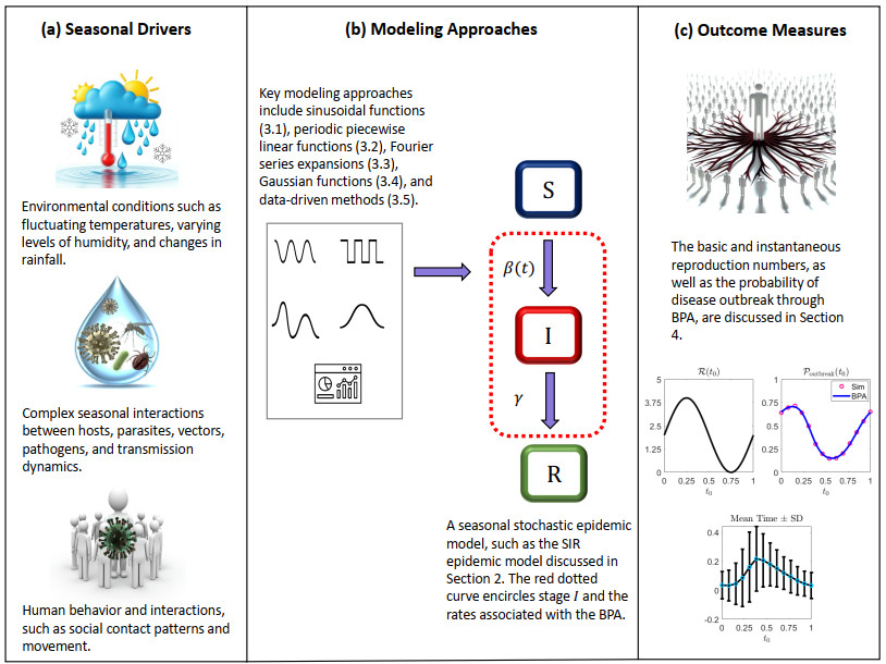
Seasonal variations in the incidence of infectious diseases are a well-established phenomenon, driven by factors such as climate changes, social behaviors, and ecological interactions that influence host susceptibility and transmission rates. While seasonality plays a significant role in shaping epidemiological dynamics, it is often overlooked in both empirical and theoretical studies. Incorporating seasonal parameters into mathematical models of infectious diseases is crucial for accurately capturing disease dynamics, enhancing the predictive power of these models, and developing successful control strategies. In this paper, I highlight key modeling approaches for incorporating seasonality into disease transmission, including sinusoidal functions, periodic piecewise linear functions, Fourier series expansions, Gaussian functions, and data-driven methods. These approaches are evaluated in terms of their flexibility, complexity, and ability to capture distinct seasonal patterns observed in real-world epidemics. A comparative analysis showcases the relative strengths and limitations of each method, supported by real-world examples. Additionally, a stochastic Susceptible-Infected-Recovered (SIR) model with seasonal transmission is demonstrated through numerical simulations. Important outcome measures, such as the basic and instantaneous reproduction numbers and the probability of a disease outbreak derived from the branching process approximation of the Markov chain, are also presented to illustrate the impact of seasonality on disease dynamics.
Citation: Mahmudul Bari Hridoy. An exploration of modeling approaches for capturing seasonal transmission in stochastic epidemic models[J]. Mathematical Biosciences and Engineering, 2025, 22(2): 324-354. doi: 10.3934/mbe.2025013
Seasonal variations in the incidence of infectious diseases are a well-established phenomenon, driven by factors such as climate changes, social behaviors, and ecological interactions that influence host susceptibility and transmission rates. While seasonality plays a significant role in shaping epidemiological dynamics, it is often overlooked in both empirical and theoretical studies. Incorporating seasonal parameters into mathematical models of infectious diseases is crucial for accurately capturing disease dynamics, enhancing the predictive power of these models, and developing successful control strategies. In this paper, I highlight key modeling approaches for incorporating seasonality into disease transmission, including sinusoidal functions, periodic piecewise linear functions, Fourier series expansions, Gaussian functions, and data-driven methods. These approaches are evaluated in terms of their flexibility, complexity, and ability to capture distinct seasonal patterns observed in real-world epidemics. A comparative analysis showcases the relative strengths and limitations of each method, supported by real-world examples. Additionally, a stochastic Susceptible-Infected-Recovered (SIR) model with seasonal transmission is demonstrated through numerical simulations. Important outcome measures, such as the basic and instantaneous reproduction numbers and the probability of a disease outbreak derived from the branching process approximation of the Markov chain, are also presented to illustrate the impact of seasonality on disease dynamics.

| [1] |
S. Altizer, A. Dobson, P. Hosseini, P. Hudson, M. Pascual, P. Rohani, Seasonality and the dynamics of infectious diseases, Ecol. Lett., 9 (2006), 467–484. https://doi.org/10.1111/j.1461-0248.2005.00879.x doi: 10.1111/j.1461-0248.2005.00879.x

|
| [2] |
D. Fisman, Seasonality of viral infections: mechanisms and unknowns, Clin. Microbiol. Infect., 18 (2012), 946–954. https://doi.org/10.1111/j.1469-0691.2012.03968.x doi: 10.1111/j.1469-0691.2012.03968.x
|
| [3] |
N. C. Grassly, C. Fraser, Seasonal infectious disease epidemiology, Proc. R. Soc. London B Biol. Sci., 273 (2006), 2541–2550. https://doi.org/10.1098/rspb.2006.3604 doi: 10.1098/rspb.2006.3604
|
| [4] |
M. E. Martinez, The calendar of epidemics: seasonal cycles of infectious diseases, PLoS Pathog., 14 (2018), e1007327. https://doi.org/10.1371/journal.ppat.1007327 doi: 10.1371/journal.ppat.1007327
|
| [5] |
L. Stone, R. Olinky, A. Huppert, Seasonal dynamics of recurrent epidemics, Nature, 446 (2007), 533–536. https://doi.org/10.1038/nature05638 doi: 10.1038/nature05638
|
| [6] |
S. Altizer, R. S. Ostfeld, P. T. J. Johnson, S. Kutz, C. D. Harvell, Climate change and infectious diseases: from evidence to a predictive framework, Science, 341 (2013), 514–519. https://doi.org/10.1126/science.1239401 doi: 10.1126/science.1239401
|
| [7] |
B. Buonomo, N. Chitnis, A. d'Onofrio, Seasonality in epidemic models: a literature review, Ric. Mate., 67 (2018), 7–25. https://doi.org/10.1007/s11587-017-0332-2 doi: 10.1007/s11587-017-0332-2
|
| [8] |
V. Andreasen, Dynamics of annual influenza a epidemics with immuno-selection, J. Math. Biol., 46 (2003), 504–536. https://doi.org/10.1007/s00285-002-0182-3 doi: 10.1007/s00285-002-0182-3
|
| [9] |
N. Chitnis, D. Hardy, T. Smith, A periodically-forced mathematical model for the seasonal dynamics of malaria in mosquitoes, Bull. Math. Biol., 74 (2012), 1098–1124. https://doi.org/10.1007/s11538-012-9696-6 doi: 10.1007/s11538-012-9696-6
|
| [10] |
G. M. A. M. Chowell, M. A. Miller, C. Viboud, Seasonal influenza in the United States, France, and Australia: transmission and prospects for control, Epidemiol. Infect., 136 (2008), 852–864. https://doi.org/10.1017/S0950268807009144 doi: 10.1017/S0950268807009144
|
| [11] |
A. K. Coussens, The role of UV radiation and vitamin D in the seasonality and outcomes of infectious disease, Photochem. Photobiol. Sci., 16 (2017), 314–338. https://doi.org/10.1039/C6PP00335A doi: 10.1039/C6PP00335A
|
| [12] |
S. F. Dowell, M. S. Ho, Seasonality of infectious diseases and severe acute respiratory syndrome–what we don't know can hurt us, Lancet Infect. Dis., 4 (2004), 704–708. https://doi.org/10.1016/S1473-3099(04)01177-6 doi: 10.1016/S1473-3099(04)01177-6
|
| [13] |
P. E. M. Fine, J. A. Clarkson, Measles in England and Wales—I: an analysis of factors underlying seasonal patterns, Int. J. Epidemiol., 11 (1982), 5–14. https://doi.org/10.1093/ije/11.1.5 doi: 10.1093/ije/11.1.5
|
| [14] | M. B. Hridoy, A. Peace, Synergizing health strategies: exploring the interplay of treatment and vaccination in an age-structured malaria model, preprint, medRxiv: 26.24314198. |
| [15] |
A. Jutla, E. Whitcombe, N. Hasan, B. Haley, A. Akanda, A. Huq, et al., Environmental factors influencing epidemic cholera, Am. J. Trop. Med. Hyg., 89 (2013), 597. https://doi.org/10.4269/ajtmh.12-0721 doi: 10.4269/ajtmh.12-0721
|
| [16] |
N. Kronfeld-Schor, T. J. Stevenson, S. Nickbakhsh, E. S. Schernhammer, X. C. Dopico, T. Dayan, et al., Drivers of infectious disease seasonality: potential implications for COVID-19, J. Biol. Rhythms, 36 (2021), 35–54. https://doi.org/10.1177/0748730420987322 doi: 10.1177/0748730420987322
|
| [17] |
W. P. London, J. A. Yorke, Recurrent outbreaks of measles, chickenpox and mumps: I. Seasonal variation in contact rates, Am. J. Epidemiol., 98 (1973), 453–468. https://doi.org/10.1093/oxfordjournals.aje.a121568 doi: 10.1093/oxfordjournals.aje.a121568
|
| [18] |
A. Nguyen, J. Mahaffy, N. K. Vaidya, Modeling transmission dynamics of Lyme disease: multiple vectors, seasonality, and vector mobility, Infect. Dis. Modell., 4 (2019), 28–43. https://doi.org/10.1016/j.idm.2019.01.001 doi: 10.1016/j.idm.2019.01.001
|
| [19] |
E. P. Pliego, J. Velázquez-Castro, A. F. Collar, Seasonality on the life cycle of Aedes aegypti mosquito and its statistical relation with dengue outbreaks, Appl. Math. Modell., 50 (2017), 484–496. https://doi.org/10.1016/j.apm.2017.05.013 doi: 10.1016/j.apm.2017.05.013
|
| [20] |
H. E. Soper, The interpretation of periodicity in disease prevalence, J. R. Stat. Soc., 92 (1929), 34–73. https://doi.org/10.2307/2341375 doi: 10.2307/2341375
|
| [21] |
W. O. Kermack, A. G. McKendrick, A contribution to the mathematical theory of epidemics, Proc. R. Soc. London Ser. A, 115 (1927), 700–721. https://doi.org/10.1098/rspa.1927.0118 doi: 10.1098/rspa.1927.0118
|
| [22] |
R. M. Anderson, Populations and infectious diseases: ecology or epidemiology?, J. Anim. Ecol., 60 (1991), 1–50. https://doi.org/10.2307/5448 doi: 10.2307/5448
|
| [23] |
J. L. Aron, I. B. Schwartz, Seasonality and period-doubling bifurcations in an epidemic model, J. Theor. Biol., 110 (1984), 665–679. https://doi.org/10.1016/S0022-5193(84)80272-4 doi: 10.1016/S0022-5193(84)80272-4
|
| [24] |
N. Bacaër, Approximation of the basic reproduction number $ R_0 $ for vector-borne diseases with a periodic vector population, Bull. Math. Biol., 69 (2007), 1067–1091. https://doi.org/10.1007/s11538-006-9166-9 doi: 10.1007/s11538-006-9166-9
|
| [25] |
L. Billings, E. Forgoston, Seasonal forcing in stochastic epidemiology models, Ric. Mate., 67 (2018), 27–47. https://doi.org/10.1007/s11587-018-0374-2 doi: 10.1007/s11587-018-0374-2
|
| [26] |
D. Gao, Y. Lou, S. Ruan, A periodic Ross-Macdonald model in a patchy environment, Discrete Contin. Dyn. Syst. Ser. B, 19 (2014), 3133. https://doi.org/10.3934/dcdsb.2014.19.3133 doi: 10.3934/dcdsb.2014.19.3133
|
| [27] |
A. Nandi, L. J. S. Allen, Probability of a zoonotic spillover with seasonal variation, Infect. Dis. Modell., 6 (2021), 514–531. https://doi.org/10.1016/j.idm.2021.06.006 doi: 10.1016/j.idm.2021.06.006
|
| [28] |
K. F. Nipa, L. J. S. Allen, Disease emergence in multi-patch stochastic epidemic models with demographic and seasonal variability, Bull. Math. Biol., 82 (2020), 152. https://doi.org/10.1007/s11538-020-00790-3 doi: 10.1007/s11538-020-00790-3
|
| [29] |
P. E. Parham, E. Michael, Modeling the effects of weather and climate change on malaria transmission, Environ. Health Perspect., 118 (2010), 620–626. https://doi.org/10.1289/ehp.0901256 doi: 10.1289/ehp.0901256
|
| [30] |
O. Prosper, K. Gurski, M. Teboh-Ewungkem, A. Peace, Z. Feng, M. Reynolds, et al., Modeling seasonal malaria transmission, Lett. Biomath., 10 (2023), 3–27. https://doi.org/10.30707/LiB10.1Prosper doi: 10.30707/LiB10.1Prosper
|
| [31] |
P. Suparit, A. Wiratsudakul, C. Modchang, A mathematical model for Zika virus transmission dynamics with a time-dependent mosquito biting rate, Theor. Biol. Med. Modell., 15 (2018), 1–11. https://doi.org/10.1186/s12976-018-0090-6 doi: 10.1186/s12976-018-0090-6
|
| [32] |
R. H. Wang, Z. Jin, Q. X. Liu, J. van de Koppel, D. Alonso, A simple stochastic model with environmental transmission explains multi-year periodicity in outbreaks of avian flu, PLoS One, 7 (2012), e28873. https://doi.org/10.1371/journal.pone.0028873 doi: 10.1371/journal.pone.0028873
|
| [33] |
X. Wang, X. Q. Zhao, Dynamics of a time-delayed Lyme disease model with seasonality, SIAM J. Appl. Dyn. Syst., 16 (2017), 853–881. https://doi.org/10.1137/16M1089373 doi: 10.1137/16M1089373
|
| [34] |
D. Y. Trejos, J. C. Valverde, E. Venturino, Dynamics of infectious diseases: a review of the main biological aspects and their mathematical translation, Appl. Math. Nonlinear Sci., 7 (2022), 1–26. https://doi.org/10.2478/amns.2022.1 doi: 10.2478/amns.2022.1
|
| [35] |
K. L. Gage, T. R. Burkot, R. J. Eisen, E. B. Hayes, Climate and vectorborne diseases, Am. J. Prev. Med., 35 (2008), 436–450. https://doi.org/10.1016/j.amepre.2008.08.030 doi: 10.1016/j.amepre.2008.08.030
|
| [36] |
R. W. Sutherst, Global change and human vulnerability to vector-borne diseases, Clin. Microbiol. Rev., 17 (2004), 136–173. https://doi.org/10.1128/CMR.17.1.136-173.2004 doi: 10.1128/CMR.17.1.136-173.2004
|
| [37] |
A. Swei, L. I. Couper, L. L. Coffey, D. Kapan, S. Bennett, Patterns, drivers, and challenges of vector-borne disease emergence, Vector-Borne Zoonotic Dis., 20 (2020), 159–170. https://doi.org/10.1089/vbz.2019.2605 doi: 10.1089/vbz.2019.2605
|
| [38] |
N. G. Becker, T. Britton, Statistical studies of infectious disease incidence, J. R. Stat. Soc. Ser. B, 61 (1999), 287–307. https://doi.org/10.1111/1467-9868.00179 doi: 10.1111/1467-9868.00179
|
| [39] |
C. F. Christiansen, L. Pedersen, H. T. Sørensen, K. J. Rothman, Methods to assess seasonal effects in epidemiological studies of infectious diseases—exemplified by application to the occurrence of meningococcal disease, Clin. Microbiol. Infect., 18 (2012), 963–969. https://doi.org/10.1111/j.1469-0691.2012.03993.x doi: 10.1111/j.1469-0691.2012.03993.x
|
| [40] |
L. Madaniyazi, A. Tobias, Y. Kim, Y. Chung, B. Armstrong, M. Hashizume, Assessing seasonality and the role of its potential drivers in environmental epidemiology: a tutorial, Int. J. Epidemiol., 51 (2022), 1677–1686. https://doi.org/10.1093/ije/dyac116 doi: 10.1093/ije/dyac116
|
| [41] | L. J. S. Allen, An introduction to stochastic epidemic models, in Mathematical Epidemiology, Springer, (2008), 81–130. https://doi.org/10.1007/978-3-540-78911-6_3 |
| [42] |
L. J. S. Allen, A primer on stochastic epidemic models: Formulation, numerical simulation, and analysis, Infect. Dis. Modell., 2 (2017), 128–142. https://doi.org/10.1016/j.idm.2017.03.001 doi: 10.1016/j.idm.2017.03.001
|
| [43] |
L. J. S. Allen, S. R. Jang, L. I. T. Roeger, Predicting population extinction or disease outbreaks with stochastic models, Lett. Biomath., 4 (2017), 1–22. https://doi.org/10.30707/LiB4.1Allen doi: 10.30707/LiB4.1Allen
|
| [44] | P. E. Greenwood, L. F. Gordillo, Stochastic epidemic modeling, in Mathematical and Statistical Estimation Approaches in Epidemiology, Springer, (2009), 31–52. https://doi.org/10.1007/978-90-481-2313-1_2 |
| [45] | M. B. Hridoy, L. J. S. Allen, Investigating seasonal disease emergence and extinction in stochastic epidemic models, Math. Biosci., 2024 (2024), forthcoming. |
| [46] |
D. T. Gillespie, Exact stochastic simulation of coupled chemical reactions, J. Phys. Chem., 81 (1977), 2340–2361. https://doi.org/10.1021/j100540a008 doi: 10.1021/j100540a008
|
| [47] |
P. Carmona, S. Gandon, Winter is coming: Pathogen emergence in seasonal environments, PLoS Comput. Biol., 16 (2020), e1007954. https://doi.org/10.1371/journal.pcbi.1007954 doi: 10.1371/journal.pcbi.1007954
|
| [48] |
A. Pandey, A. Mubayi, J. Medlock, Comparing vector–host and SIR models for dengue transmission, Math. Biosci., 246 (2013), 252–259. https://doi.org/10.1016/j.mbs.2013.02.008 doi: 10.1016/j.mbs.2013.02.008
|
| [49] |
X. Tan, L. Yuan, J. Zhou, Y. Zheng, F. Yang, Modeling the initial transmission dynamics of influenza A H1N1 in Guangdong province, China, Int. J. Infect. Dis., 17 (2013), e479–e484. https://doi.org/10.1016/j.ijid.2012.12.022 doi: 10.1016/j.ijid.2012.12.022
|
| [50] | J. B. J. B. Fourier, The Analytical Theory of Heat, Courier Corporation, 2003. https://doi.org/10.5962/bhl.title.55578 |
| [51] |
L. J. S. Allen, X. Wang, Stochastic models of infectious diseases in a periodic environment with application to cholera epidemics, J. Math. Biol., 82 (2021), 48. https://doi.org/10.1007/s00285-020-01526-4 doi: 10.1007/s00285-020-01526-4
|
| [52] |
J. P. Chávez, T. Götz, S. Siegmund, K. P. Wijaya, An SIR-dengue transmission model with seasonal effects and impulsive control, Math. Biosci., 289 (2017), 29–39. https://doi.org/10.1016/j.mbs.2017.04.003 doi: 10.1016/j.mbs.2017.04.003
|
| [53] |
J. Huang, S. Ruan, X. Wu, X. Zhou, Seasonal transmission dynamics of measles in China, Theory Biosci., 137 (2018), 185–195. https://doi.org/10.1007/s12064-018-0267-y doi: 10.1007/s12064-018-0267-y
|
| [54] |
K. Husar, D. C. Pittman, J. Rajala, F. Mostafa, L. J. S. Allen, Lyme disease models of tick-mouse dynamics with seasonal variation in births, deaths, and tick feeding, Bull. Math. Biol., 86 (2024), 25. https://doi.org/10.1007/s11538-024-01033-9 doi: 10.1007/s11538-024-01033-9
|
| [55] |
M. Kamo, A. Sasaki, The effect of cross-immunity and seasonal forcing in a multi-strain epidemic model, Phys. D Nonlinear Phenom., 165 (2002), 228–241. https://doi.org/10.1016/S0167-2789(02)00386-4 doi: 10.1016/S0167-2789(02)00386-4
|
| [56] |
X. Liu, J. Huang, C. Li, Y. Zhao, D. Wang, Z. Huang, et al., The role of seasonality in the spread of COVID-19 pandemic, Environ. Res., 195 (2021), 110874. https://doi.org/10.1016/j.envres.2021.110874 doi: 10.1016/j.envres.2021.110874
|
| [57] |
A. L. Lloyd, R. M. May, Spatial heterogeneity in epidemic models, J. Theor. Biol., 179 (1996), 1–11. https://doi.org/10.1006/jtbi.1996.0049 doi: 10.1006/jtbi.1996.0049
|
| [58] |
K. F. Nipa, L. J. S. Allen, The effect of demographic variability and periodic fluctuations on disease outbreaks in a vector-host epidemic model, Infect. Dis. Planet, 2021 (2021), 15–35. https://doi.org/10.1007/s11676-021-01319-6 doi: 10.1007/s11676-021-01319-6
|
| [59] |
S. L. Jing, H. F. Huo, H. Xiang, Modeling the effects of meteorological factors and unreported cases on seasonal influenza outbreaks in Gansu province, China, Bull. Math. Biol., 82 (2020), 1–36. https://doi.org/10.1007/s11538-019-00671-6 doi: 10.1007/s11538-019-00671-6
|
| [60] | Average monthly temperature in the United States from January 2020 to July 2024, 2024. Available from: https://www.statista.com/statistics/513628/monthly-average-temperature-in-the-us-fahrenheit/. |
| [61] | Centers for Disease Control and Prevention (CDC), 2023. Available from: https://gis.cdc.gov/grasp/fluview/fluportaldashboard.html. |
| [62] |
A. d'Onofrio, J. Duarte, C. Januário, N. Martins, A SIR forced model with interplays with the external world and periodic internal contact interplays, Phys. Lett. A, 454 (2022), 128498. https://doi.org/10.1016/j.physleta.2022.128498 doi: 10.1016/j.physleta.2022.128498
|
| [63] |
G. González-Parra, A. J. Arenas, L. Jódar, Piecewise finite series solutions of seasonal diseases models using multistage Adomian method, Commun. Nonlinear Sci. Numer. Simul., 14 (2009), 3967–3977. https://doi.org/10.1016/j.cnsns.2009.02.023 doi: 10.1016/j.cnsns.2009.02.023
|
| [64] |
C. J. Silva, G. Cantin, C. Cruz, R. Fonseca-Pinto, R. Passadouro, E. S. Dos Santos, et al., Complex network model for COVID-19: human behavior, pseudo-periodic solutions and multiple epidemic waves, J. Math. Anal. Appl., 514 (2022), 125171. https://doi.org/10.1016/j.jmaa.2021.125171 doi: 10.1016/j.jmaa.2021.125171
|
| [65] |
R. Olinky, A. Huppert, L. Stone, Seasonal dynamics and thresholds governing recurrent epidemics, J. Math. Biol., 56 (2008), 827–839. https://doi.org/10.1007/s00285-007-0131-6 doi: 10.1007/s00285-007-0131-6
|
| [66] |
G. Tanaka, K. Aihara, Effects of seasonal variation patterns on recurrent outbreaks in epidemic models, J. Theor. Biol., 317 (2013), 87–95. https://doi.org/10.1016/j.jtbi.2012.09.005 doi: 10.1016/j.jtbi.2012.09.005
|
| [67] |
J. Zhang, Y. Li, Z. Jin, H. Zhu, Dynamics analysis of an avian influenza A (H7N9) epidemic model with vaccination and seasonality, Complexity, 2019 (2019), 4161287. https://doi.org/10.1155/2019/4161287 doi: 10.1155/2019/4161287
|
| [68] | Health Information Platform for the Americas (PLISA), Zika indicators, 2023. Available from: http://www.paho.org/data/index.php/en/?option=com_content&view=article&id=524&Itemid=. |
| [69] |
V. Capasso, G. Serio, A generalization of the Kermack-McKendrick deterministic epidemic model, Math. Biosci., 42 (1978), 43–61. https://doi.org/10.1016/0025-5564(78)90006-4 doi: 10.1016/0025-5564(78)90006-4
|
| [70] |
G. Rohith, K. B. Devika, Dynamics and control of COVID-19 pandemic with nonlinear incidence rates, Nonlinear Dyn., 101 (2020), 2013–2026. https://doi.org/10.1007/s11071-020-05935-3 doi: 10.1007/s11071-020-05935-3
|
| [71] |
T. Gavenčiak, J. T. Monrad, G. Leech, M. Sharma, S. Mindermann, S. Bhatt, et al., Seasonal variation in SARS-CoV-2 transmission in temperate climates: A Bayesian modelling study in 143 European regions, PLoS Comput. Biol., 18 (2022), e1010435. https://doi.org/10.1371/journal.pcbi.1010435 doi: 10.1371/journal.pcbi.1010435
|
| [72] | S. Deguen, G. Thomas, N. P. Chau, Estimation of the contact rate in a seasonal SEIR model: Application to chickenpox incidence in France, Stat. Med., 19 (2000), 1207–1216. |
| [73] | P. Mortensen, K. Lauer, S. P. Rautenbach, M. Gallotta, N. Sharapova, I. Takkides, et al., A machine learning-enabled SIR model for adaptive and dynamic forecasting of COVID-19, preprint, medRxiv: 30.24311170. |
| [74] | Centers for Disease Control and Prevention, Lyme disease surveillance data, 2024. Available from: https://www.cdc.gov/lyme/data-research/facts-stats/surveillance-data-1.html. |
| [75] |
S. Kumar, A. Ahmadian, R. Kumar, D. Kumar, J. Singh, D. Baleanu, et al., An efficient numerical method for fractional SIR epidemic model of infectious disease by using Bernstein wavelets, Mathematics, 8 (2020), 558. https://doi.org/10.3390/math8040558 doi: 10.3390/math8040558
|
| [76] |
L. M. Stolerman, D. Coombs, S. Boatto, SIR-network model and its application to dengue fever, SIAM J. Appl. Math., 75 (2015), 2581–2609. https://doi.org/10.1137/15M1016526 doi: 10.1137/15M1016526
|
| [77] |
M. C. Ramírez-Soto, J. V. Bogado Machuca, D. H. Stalder, D. Champin, M. G. Martínez-Fernández, et al., SIR-SI model with a Gaussian transmission rate: Understanding the dynamics of dengue outbreaks in Lima, Peru, PLoS One, 18 (2023), e0284263. https://doi.org/10.1371/journal.pone.0284263 doi: 10.1371/journal.pone.0284263
|
| [78] |
F. S. Alshammari, Analysis of SIRVI model with time-dependent coefficients and the effect of vaccination on the transmission rate and COVID-19 epidemic waves, Infect. Dis. Modell., 8 (2023), 172–182. https://doi.org/10.1016/j.idm.2023.04.002 doi: 10.1016/j.idm.2023.04.002
|
| [79] |
M. Arquam, A. Singh, H. Cherifi, Impact of seasonal conditions on vector-borne epidemiological dynamics, IEEE Access, 8 (2020), 94510–94525. https://doi.org/10.1109/ACCESS.2020.2993924 doi: 10.1109/ACCESS.2020.2993924
|
| [80] |
S. Setianto, D. Hidayat, Modeling the time-dependent transmission rate using Gaussian pulses for analyzing the COVID-19 outbreaks in the world, Sci. Rep., 13 (2023), 4466. https://doi.org/10.1038/s41598-023-31528-9 doi: 10.1038/s41598-023-31528-9
|
| [81] | M. B. Hridoy, S. M. Mustaquim, Data-driven modeling of seasonal dengue dynamics in Bangladesh: A Bayesian-stochastic approach, preprint, arXiv: 2410.00947. |
| [82] | Bangladesh Meteorological Department, normal monthly rainfall, 2023. Available from: https://live6.bmd.gov.bd//p/Normal-Monthly-Rainfall. |
| [83] | Directorate General of Health Services (DGHS), Bangladesh, daily dengue status report, 2024. Available from: https://old.dghs.gov.bd/index.php/bd/home/5200-daily-dengue-status-report. |
| [84] |
D. De Angelis, A. M. Presanis, P. J. Birrell, G. Scalia Tomba, T. House, Four key challenges in infectious disease modelling using data from multiple sources, Epidemics, 10 (2015), 83–87. https://doi.org/10.1016/j.epidem.2014.09.006 doi: 10.1016/j.epidem.2014.09.006
|
| [85] |
C. Anastassopoulou, L. Russo, A. Tsakris, C. Siettos, Data-based analysis, modelling and forecasting of the COVID-19 outbreak, PLoS One, 15 (2020), e0230405. https://doi.org/10.1371/journal.pone.0230405 doi: 10.1371/journal.pone.0230405
|
| [86] |
Y. Fang, Y. Nie, M. Penny, Transmission dynamics of the COVID-19 outbreak and effectiveness of government interventions: A data-driven analysis, J. Med. Virol., 92 (2020), 645–659. https://doi.org/10.1002/jmv.25750 doi: 10.1002/jmv.25750
|
| [87] |
E. Kuhl, Data-driven modeling of COVID-19—lessons learned, Extreme Mech. Lett., 40 (2020), 100921. https://doi.org/10.1016/j.eml.2020.100921 doi: 10.1016/j.eml.2020.100921
|
| [88] |
K. N. Nabi, Forecasting COVID-19 pandemic: A data-driven analysis, Chaos Solitons Fractals, 139 (2020), 110046. https://doi.org/10.1016/j.chaos.2020.110046 doi: 10.1016/j.chaos.2020.110046
|
| [89] |
I. Berry, M. Rahman, M. S. Flora, T. Shirin, A. S. M. Alamgir, M. H. Khan, et al., Seasonality of influenza and coseasonality with avian influenza in Bangladesh, 2010–19: A retrospective, time-series analysis, Lancet Global Health, 10 (2022), e1150–e1158. https://doi.org/10.1016/S2214-109X(22)00255-0 doi: 10.1016/S2214-109X(22)00255-0
|
| [90] |
L. C. Brooks, D. C. Farrow, S. Hyun, R. J. Tibshirani, R. Rosenfeld, Flexible modeling of epidemics with an empirical Bayes framework, PLoS Comput. Biol., 11 (2015), e1004382. https://doi.org/10.1371/journal.pcbi.1004382 doi: 10.1371/journal.pcbi.1004382
|
| [91] |
N. Chintalapudi, G. Battineni, F. Amenta, COVID-19 virus outbreak forecasting of registered and recovered cases after sixty-day lockdown in Italy: A data-driven model approach, J. Microbiol. Immunol. Infect., 53 (2020), 396–403. https://doi.org/10.1016/j.jmii.2020.04.004 doi: 10.1016/j.jmii.2020.04.004
|
| [92] |
J. Dawa, G. O. Emukule, E. Barasa, M. A. Widdowson, O. Anzala, E. Van Leeuwen, et al., Seasonal influenza vaccination in Kenya: An economic evaluation using dynamic transmission modelling, BMC Med., 18 (2020), 19. https://doi.org/10.1186/s12916-019-1473-6 doi: 10.1186/s12916-019-1473-6
|
| [93] |
F. O. Ochieng, SEIRS model for malaria transmission dynamics incorporating seasonality and awareness campaign, Infect. Dis. Modell., 9 (2024), 84–102. https://doi.org/10.1016/j.idm.2024.01.001 doi: 10.1016/j.idm.2024.01.001
|
| [94] |
J. M. Read, J. R. E. Bridgen, D. A. T. Cummings, A. Ho, C. P. Jewell, Novel coronavirus 2019-nCoV (COVID-19): Early estimation of epidemiological parameters and epidemic size estimates, Philos. Transact. R. Soc. B, 376 (2021), 20200265. https://doi.org/10.1098/rstb.2020.0265 doi: 10.1098/rstb.2020.0265
|
| [95] |
H. Yuan, S. C. Kramer, E. H. Y. Lau, B. J. Cowling, W. Yang, Modeling influenza seasonality in the tropics and subtropics, PLoS Comput. Biol., 17 (2021), e1009050. https://doi.org/10.1371/journal.pcbi.1009050 doi: 10.1371/journal.pcbi.1009050
|
| [96] |
C. E. McCulloch, Generalized linear models, J. Am. Stat. Assoc., 95 (2000), 1320–1324. https://doi.org/10.1080/01621459.2000.10474315 doi: 10.1080/01621459.2000.10474315
|
| [97] | T. J. Hastie, Generalized additive models, in Statistical Models in S, Routledge, (2017), 249–307. |
| [98] |
E. Ostertagová, Modelling using polynomial regression, Proc. Eng., 48 (2012), 500–506. https://doi.org/10.1016/j.proeng.2012.09.545 doi: 10.1016/j.proeng.2012.09.545
|
| [99] |
M. N. Alenezi, F. S. Al-Anzi, H. Alabdulrazzaq, Building a sensible SIR estimation model for COVID-19 outspread in Kuwait, Alex. Eng. J., 60 (2021), 3161–3175. https://doi.org/10.1016/j.aej.2021.02.048 doi: 10.1016/j.aej.2021.02.048
|
| [100] |
A. Capaldi, S. Behrend, B. Berman, J. Smith, J. Wright, A. L. Lloyd, Parameter estimation and uncertainty quantification for an epidemic model, Math. Biosci. Eng., 9 (2012), 553–576. https://doi.org/10.3934/mbe.2012.9.553 doi: 10.3934/mbe.2012.9.553
|
| [101] |
I. J. Myung, Tutorial on maximum likelihood estimation, J. Math. Psychol., 47 (2003), 90–100. https://doi.org/10.1016/S0022-2496(02)00028-7 doi: 10.1016/S0022-2496(02)00028-7
|
| [102] |
L. M. A. Bettencourt, R. M. Ribeiro, Real time Bayesian estimation of the epidemic potential of emerging infectious diseases, PLoS One, 3 (2008), e2185. https://doi.org/10.1371/journal.pone.0002185 doi: 10.1371/journal.pone.0002185
|
| [103] |
F. S. Tabataba, P. Chakraborty, N. Ramakrishnan, S. Venkatramanan, J. Chen, B. Lewis, et al., A framework for evaluating epidemic forecasts, BMC Infect. Dis., 17 (2017), 1–27. https://doi.org/10.1186/s12879-017-2764-9 doi: 10.1186/s12879-017-2764-9
|
| [104] |
M. Ajelli, B. Gonçalves, D. Balcan, V. Colizza, H. Hu, J. J. Ramasco, et al., Comparing large-scale computational approaches to epidemic modeling: Agent-based versus structured metapopulation models, BMC Infect. Dis., 10 (2010), 1–13. https://doi.org/10.1186/1471-2334-10-190 doi: 10.1186/1471-2334-10-190
|
| [105] |
T. L. Wiemken, R. R. Kelley, Machine learning in epidemiology and health outcomes research, Ann. Rev. Public Health, 41 (2020), 21–36. https://doi.org/10.1146/annurev-publhealth-040119-094437 doi: 10.1146/annurev-publhealth-040119-094437
|
| [106] |
A. Rodríguez, H. Kamarthi, P. Agarwal, J. Ho, M. Patel, S. Sapre, et al., Machine learning for data-centric epidemic forecasting, Nat. Mach. Intell., 6 (2024), 1–10. https://doi.org/10.1038/s42256-024-00678-5 doi: 10.1038/s42256-024-00678-5
|
| [107] |
O. Diekmann, J. A. P. Heesterbeek, J. A. J. Metz, On the definition and the computation of the basic reproduction ratio $R_0$ in models for infectious diseases in heterogeneous populations, J. Math. Biol., 28 (1990), 365–382. https://doi.org/10.1007/BF00178324 doi: 10.1007/BF00178324
|
| [108] |
W. Wang, X. Zhao, Threshold dynamics for compartmental epidemic models in periodic environments, J. Dyn. Differ. Equations, 20 (2008), 699–717. https://doi.org/10.1007/s10884-008-9109-3 doi: 10.1007/s10884-008-9109-3
|
| [109] |
C. A. Klausmeier, Floquet theory: A useful tool for understanding nonequilibrium dynamics, Theor. Ecol., 1 (2008), 153–161. https://doi.org/10.1007/s12080-008-0014-y doi: 10.1007/s12080-008-0014-y
|
| [110] |
O. Diekmann, J. A. P. Heesterbeek, M. G. Roberts, The construction of next-generation matrices for compartmental epidemic models, J. R. Soc. Int., 7 (2010), 873–885. https://doi.org/10.1098/rsif.2009.0386 doi: 10.1098/rsif.2009.0386
|
| [111] |
K. Dietz, The estimation of the basic reproduction number for infectious diseases, Stat. Methods Med. Res., 2 (1993), 23–41. https://doi.org/10.1177/096228029300200103 doi: 10.1177/096228029300200103
|
| [112] |
P. Van den Driessche, Reproduction numbers of infectious disease models, Infect. Dis. Modell., 2 (2017), 288–303. https://doi.org/10.1016/j.idm.2017.06.002 doi: 10.1016/j.idm.2017.06.002
|
| [113] |
L. J. S. Allen, G. E. Lahodny Jr., Extinction thresholds in deterministic and stochastic epidemic models, J. Biol. Dyn., 6 (2012), 590–611. https://doi.org/10.1080/17513758.2012.716436 doi: 10.1080/17513758.2012.716436
|
| [114] |
N. Bacaër, E. H. Ait Dads, On the probability of extinction in a periodic environment, J. Math. Biol., 68 (2014), 533–548. https://doi.org/10.1007/s00285-013-0655-7 doi: 10.1007/s00285-013-0655-7
|
| [115] |
F. Ball, The threshold behaviour of epidemic models, J. Appl. Prob., 20 (1983), 227–241. https://doi.org/10.2307/3213746 doi: 10.2307/3213746
|
| [116] |
O. M. Otunuga, Global stability of nonlinear stochastic SEI epidemic model with fluctuations in transmission rate of disease, Int. J. Stochastic Anal., 2017 (2017), 6313620. https://doi.org/10.1155/2017/6313620 doi: 10.1155/2017/6313620
|
| [117] |
J. Rashidinia, M. Sajjadian, J. Duarte, C. Januário, N. Martins, On the dynamical complexity of a seasonally forced discrete SIR epidemic model with a constant vaccination strategy, Complexity, 2018 (2018), 7191487. https://doi.org/10.1155/2018/7191487 doi: 10.1155/2018/7191487
|
| [118] |
M. S. Tackney, T. Morris, I. White, C. Leyrat, K. Diaz-Ordaz, E. Williamson, A comparison of covariate adjustment approaches under model misspecification in individually randomized trials, Trials, 24 (2023), 14. https://doi.org/10.1186/s13063-022-06986-4 doi: 10.1186/s13063-022-06986-4
|
| [119] |
P. Glendinning, L. P. Perry, Melnikov analysis of chaos in a simple epidemiological model, J. Math. Biol., 35 (1997), 359–373. https://doi.org/10.1007/s002850050057 doi: 10.1007/s002850050057
|
| [120] |
D. He, D. J. D. Earn, Epidemiological effects of seasonal oscillations in birth rates, Theor. Popul. Biol., 72 (2007), 274–291. https://doi.org/10.1016/j.tpb.2007.05.004 doi: 10.1016/j.tpb.2007.05.004
|
| [121] |
K. F. Nipa, S. R. J. Jang, L. J. S. Allen, The effect of demographic and environmental variability on disease outbreak for a dengue model with a seasonally varying vector population, Math. Biosci., 331 (2021), 108516. https://doi.org/10.1016/j.mbs.2020.108516 doi: 10.1016/j.mbs.2020.108516
|
| [122] |
I. B. Schwartz, H. L. Smith, Infinite subharmonic bifurcation in an SEIR epidemic model, J. Math. Biol., 18 (1983), 233–253. https://doi.org/10.1007/BF00276314 doi: 10.1007/BF00276314
|


Figures(11) / Tables(2)

Mahmudul Bari Hridoy. An exploration of modeling approaches for capturing seasonal transmission in stochastic epidemic models[J]. Mathematical Biosciences and Engineering, 2025, 22(2): 324-354. doi: 10.3934/mbe.2025013


 DownLoad: