Non-spatial models of competition between floating aquatic vegetation (FAV) and submersed aquatic vegetation (SAV) predict a stable state of pure SAV at low total available limiting nutrient level, N, a stable state of only FAV for high N, and alternative stable states for intermediate N, as described by an S-shaped bifurcation curve. Spatial models that include physical heterogeneity of the waterbody show that the sharp transitions between these states become smooth. We examined the effects of heterogeneous initial conditions of the vegetation types. We used a spatially explicit model to describe the competition between the vegetation types. In the model, the FAV, duckweed (L. gibba), competed with the SAV, Nuttall's waterweed (Elodea nuttallii). Differences in the initial establishment of the two macrophytes affected the possible stable equilibria. When initial biomasses of SAV and FAV differed but each had the same initial biomass in each spatial cell, the S-shaped bifurcation resulted, but the critical transitions on the N-axis are shifted, depending on FAV:SAV biomass ratio. When the initial biomasses of SAV and FAV were randomly heterogeneously distributed among cells, the vegetation pattern of the competing species self-organized spatially, such that many different stable states were possible in the intermediate N region. If N was gradually increased or decreased through time from a stable state, the abrupt transitions of non-spatial models were changed into smoother transitions through a series of stable states, which resembles the Busse balloon observed in other systems.
Citation: Linhao Xu, Donald L. DeAngelis. Effects of initial vegetation heterogeneity on competition of submersed and floating macrophytes[J]. Mathematical Biosciences and Engineering, 2024, 21(10): 7194-7210. doi: 10.3934/mbe.2024318
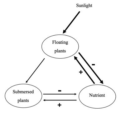
Non-spatial models of competition between floating aquatic vegetation (FAV) and submersed aquatic vegetation (SAV) predict a stable state of pure SAV at low total available limiting nutrient level, N, a stable state of only FAV for high N, and alternative stable states for intermediate N, as described by an S-shaped bifurcation curve. Spatial models that include physical heterogeneity of the waterbody show that the sharp transitions between these states become smooth. We examined the effects of heterogeneous initial conditions of the vegetation types. We used a spatially explicit model to describe the competition between the vegetation types. In the model, the FAV, duckweed (L. gibba), competed with the SAV, Nuttall's waterweed (Elodea nuttallii). Differences in the initial establishment of the two macrophytes affected the possible stable equilibria. When initial biomasses of SAV and FAV differed but each had the same initial biomass in each spatial cell, the S-shaped bifurcation resulted, but the critical transitions on the N-axis are shifted, depending on FAV:SAV biomass ratio. When the initial biomasses of SAV and FAV were randomly heterogeneously distributed among cells, the vegetation pattern of the competing species self-organized spatially, such that many different stable states were possible in the intermediate N region. If N was gradually increased or decreased through time from a stable state, the abrupt transitions of non-spatial models were changed into smoother transitions through a series of stable states, which resembles the Busse balloon observed in other systems.

| [1] |
M. Scheffer, S. Szabo, A. Gragnani, E. Van Nes, S. Rinaldi, N. Kautsky, et al., Floating plant dominance as a stable state, PNAS, 100 (2003), 4040−4045. https://doi.org/10.1073/pnas.0737918100 doi: 10.1073/pnas.0737918100

|
| [2] |
E. van Nes, M. Scheffer, Implications of spatial heterogeneity for catastrophic regime shifts in ecosystems, Ecology, 86 (2005), 1797−1807. https://doi.org/10.1890/04-0550 doi: 10.1890/04-0550
|
| [3] |
M. McCann, Evidence of alternative states in freshwater lakes: A spatially-explicit model of submerged and floating plants, Ecol. Modell., 337 (2016), 298−309. https://doi.org/10.1016/j.ecolmodel.2016.07.006 doi: 10.1016/j.ecolmodel.2016.07.006
|
| [4] |
L. Xu, D. L. DeAngelis, Spatial patterns as long transients in submersed-floating plant competition with biocontrol, Theor Ecol., (2024). https://doi.org/10.1007/s12080-024-00584-6 doi: 10.1007/s12080-024-00584-6
|
| [5] |
A. B. Janssen, D. van Wijk, L. P. Van Gerven, E. S. Bakker, R. J. Brederveld, D. L. DeAngelis, et al., Success of lake restoration depends on spatial aspects of nutrient loading and hydrology, Sci. Tot. Envir., 679 (2019), 248−259. https://doi.org/10.1016/j.scitotenv.2019.04.4430048-9697 doi: 10.1016/j.scitotenv.2019.04.4430048-9697
|
| [6] |
M. Rietkerk, R. Bastiaansen, S. Banerjee, J. van de Koppel, M. Baudena, A. Doelman, Evasion of tipping in complex systems through spatial pattern formation, Science, 374 (2021). https://doi.org/10.1126/science.abj0359 doi: 10.1126/science.abj0359
|
| [7] |
S. Kéfi, A. Génin, A. Garcia-Mayor, E. Guirado, J. S. Cabral, M. Berdugo, et al., Self-organization as a mechanism of resilience in dryland ecosystems, PNAS, 121 (2024), p.e2305153121. https://doi.org/10.1073/pnas.2305153121 doi: 10.1073/pnas.2305153121
|
| [8] |
R. Bastiaansen, O. Jaïbi, V. Deblauwe, M. Eppinga, K. Siteur, E. Siero, et al., Multistability of model and real dryland ecosystems through spatial self-organization, PNAS, 115 (2018), 11256−11261. https://doi.org/10.1073/pnas.1804771115 doi: 10.1073/pnas.1804771115
|
| [9] |
R. Bastiaansen, H. Dijkstra, A. von der Heydt, Fragmented tipping in a spatially heterogeneous world, Environ. Res. Lett., 17 (2022). https://doi.org/10.1088/1748-9326/ac59a8 doi: 10.1088/1748-9326/ac59a8
|
| [10] |
M. Rietkerk, J. van de Koppel, Regular pattern formation in real ecosystems, Trends Ecol. Evol., 23 (2008), 169−175. https://doi.org/10.1016/j.tree.2007.10.013 doi: 10.1016/j.tree.2007.10.013
|
| [11] | J. von Hardenberg, E. Meron, M. Shachak, Y. Zarmi, Diversity of vegetation patterns and desertification, Phys. Rev. Lett., 87 (2001), 198101. https://doi-org.access.library.miami.edu/10.1103/PhysRevLett.87.198101 |
| [12] |
K. Siteur, E. Siero, M. Eppinga, J. Rademacher, A. Doelman, M. Rietkerk, Beyond Turing: The response of patterned ecosystems to environmental change, Ecol. Complex., 20 (2014), 81−96. https://doi.org/10.1016/j.ecocom.2014.09.002 doi: 10.1016/j.ecocom.2014.09.002
|
| [13] |
A.Vanselow, L. Halekotte, P. Pal, S. Wieczorek, U. Feudel, Rate-induced tipping can trigger plankton blooms, Theor. Ecol., 17 (2024), 1−7. https://doi.org/10.1007/s12080-024-00577-5 doi: 10.1007/s12080-024-00577-5
|
| [14] |
E. Sheffer, J. von Hardenberg, H. Yizhaq, M. Shachak, E. Meron, Emerged or imposed: A theory on the role of physical templates and self‐organisation for vegetation patchiness, Ecol. Lett., 16 (2013), 127−139. http://doi.org/10.1111/ele.12027 doi: 10.1111/ele.12027
|
| [15] |
X. Dong, S. Fisher, Ecosystem spatial self-organization: free order for nothing?, Ecol. Complex., 38 (2019), 24−30. https://doi.org/10.1016/j.ecocom.2019.01.002 doi: 10.1016/j.ecocom.2019.01.002
|


Figures(10) / Tables(1)

Linhao Xu, Donald L. DeAngelis. Effects of initial vegetation heterogeneity on competition of submersed and floating macrophytes[J]. Mathematical Biosciences and Engineering, 2024, 21(10): 7194-7210. doi: 10.3934/mbe.2024318


 DownLoad: