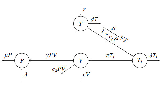
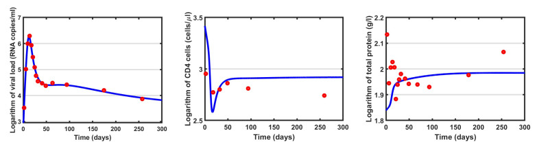
In this paper we develop a four compartment within-host model of nutrition and HIV. We show that the model has two equilibria: an infection-free equilibrium and infection equilibrium. The infection free equilibrium is locally asymptotically stable when the basic reproduction number $ \mathcal{R}_0 < 1 $, and unstable when $ \mathcal{R}_0 > 1 $. The infection equilibrium is locally asymptotically stable if $ \mathcal{R}_0 > 1 $ and an additional condition holds. We show that the within-host model of HIV and nutrition is structured to reveal its parameters from the observations of viral load, CD4 cell count and total protein data. We then estimate the model parameters for these 3 data sets. We have also studied the practical identifiability of the model parameters by performing Monte Carlo simulations, and found that the rate of clearance of the virus by immunoglobulins is practically unidentifiable, and that the rest of the model parameters are only weakly identifiable given the experimental data. Furthermore, we have studied how the data frequency impacts the practical identifiability of model parameters.
Citation: Archana N. Timsina, Yuganthi R. Liyanage, Maia Martcheva, Necibe Tuncer. A novel within-host model of HIV and nutrition[J]. Mathematical Biosciences and Engineering, 2024, 21(4): 5577-5603. doi: 10.3934/mbe.2024246
In this paper we develop a four compartment within-host model of nutrition and HIV. We show that the model has two equilibria: an infection-free equilibrium and infection equilibrium. The infection free equilibrium is locally asymptotically stable when the basic reproduction number $ \mathcal{R}_0 < 1 $, and unstable when $ \mathcal{R}_0 > 1 $. The infection equilibrium is locally asymptotically stable if $ \mathcal{R}_0 > 1 $ and an additional condition holds. We show that the within-host model of HIV and nutrition is structured to reveal its parameters from the observations of viral load, CD4 cell count and total protein data. We then estimate the model parameters for these 3 data sets. We have also studied the practical identifiability of the model parameters by performing Monte Carlo simulations, and found that the rate of clearance of the virus by immunoglobulins is practically unidentifiable, and that the rest of the model parameters are only weakly identifiable given the experimental data. Furthermore, we have studied how the data frequency impacts the practical identifiability of model parameters.

| [1] |
A. S. Perelson, P. W. Nelson, Mathematical analysis of HIV-1 dynamics in vivo, SIAM Rev., 41 (1999), 3–44. https://doi.org/10.1137/S0036144598335107 doi: 10.1137/S0036144598335107

|
| [2] | M. Nowal, R. M. May, Virus dynamics: mathematical principles of immunology and virology, Oxford University Press, Oxford, 2000. |
| [3] |
A. S. Perelson, R. M. Ribeiro, Modeling the within-host dynamics of HIV infection, BMC Biol., 11 (2013), 1–10. https://doi.org/10.1186/1741-7007-11-96 doi: 10.1186/1741-7007-11-96
|
| [4] | G. W. Nelson, A. S. Perelson, A mechanism of immune escape by slow-replicating HIV strains, J. Acq. Imm. Def., 5 (1992), 82–93. |
| [5] |
A. S. Perelson, D. E. Kirschner, R. D. Boer, Dynamics of HIV infection of CD4+ T cells, Math. Biosci., 114 (1993), 81–125. https://doi.org/10.1016/0025-5564(93)90043-A doi: 10.1016/0025-5564(93)90043-A
|
| [6] |
L. Rong, A. S. Perelson, Modeling HIV persistence, the latent reservoir, and viral blips, J. Theor. Biol., 260 (2009), 308–331. https://doi.org/10.1016/j.jtbi.2009.06.011 doi: 10.1016/j.jtbi.2009.06.011
|
| [7] |
N. K. Vaidya, R. M. Ribeiro, A. S. Perelson, A. Kumar, Modeling the effects of morphine on simian immunodeficiency virus dynamics, PLoS Comput. Biol., 12 (2016), e1005127. https://doi.org/10.1371/journal.pcbi.1005127 doi: 10.1371/journal.pcbi.1005127
|
| [8] |
M. A. Stafford, L. Corey, Y. Cao, E. S. Daar, D. D. Ho, A. S. Perelson, Modeling plasma virus concentration during primary HIV infection, J. Theor. Biol., 203 (2000), 285–301. https://doi.org/10.1006/jtbi.2000.1076 doi: 10.1006/jtbi.2000.1076
|
| [9] | A. S. Perelson, P. W. Nelson, Modeling viral infections, in Proceedings of Symposia in Applied Mathematics, 59 (2002), 139–172. |
| [10] | R. Patil, U. Raghuwanshi, Serum protein, albumin, globulin levels, and A/G ratio in HIV positive patients, Biomed. Pharmacol. J., 2 (2009), 321–325. |
| [11] |
V. T. Sowmyanarayanan, S. Jun, A. Cowan, R. L. Bailey, The nutritional status of HIV-Infected US adults, Curr. Dev. Nutr., 1 (2017), e001636. https://doi.org/10.3945/cdn.117.001636 doi: 10.3945/cdn.117.001636
|
| [12] | R. K. Chandra, Nutrition and immunity: Ⅰ. Basic considerations. Ⅱ. Practical applications, ASDC J. Dent. Child., 54 (1987), 193–197. |
| [13] | W. R. Beisel, Nutrition in pediatric HIV infection: setting the research agenda, J. Nutr., 126 (1996), 2611–2615. |
| [14] |
O. O. Oguntibeju, W. M. Van den Heever, F. E. Van Schalkwyk, The interrelationship between nutrition and the immune system in HIV infection: a review, Pak. J. Biol. Sci., 10 (2007), 4327–4338. https://doi.org/10.3923/pjbs.2007.4327.4338 doi: 10.3923/pjbs.2007.4327.4338
|
| [15] |
M. A. Eller, N. Goonetilleke, B. Tassaneetrithep, L. A. Eller, M. C. Costanzo, S. Johnson, et al., Expansion of inefficient HIV-specific CD8 T cells during acute infection, J. Virol., 90 (2016), 4005–4016. https://doi.org/10.1128/jvi.02785-15 doi: 10.1128/jvi.02785-15
|
| [16] |
T. Were, J. O. Jesca, E. Munde, C. Ouma, T. M. Titus, F. Ongecha-Owuor, et al., Clinical chemistry profiles in injection heroin users from Coastal Region, Kenya, BMC Clin. Pathol., 14 (2014), 1–9. https://doi.org/10.1186/1472-6890-14-32 doi: 10.1186/1472-6890-14-32
|
| [17] |
N. Tuncer, T. T. Le, Structural and practical identifiability analysis of outbreak models, Math. Biosci., 299 (2018), 1–18. https://doi.org/10.1016/j.mbs.2018.02.004 doi: 10.1016/j.mbs.2018.02.004
|
| [18] |
N. Tuncer, M. Marctheva, B. LaBarre, S. Payoute, Structural and practical identifiability analysis of Zika epidemiological models, Bull. Math. Biol., 80 (2018), 2209–2241. https://doi.org/10.1007/s11538-018-0453-z doi: 10.1007/s11538-018-0453-z
|
| [19] |
N. Tuncer, A. Timsina, M. Nuno, G. Chowell, M. Martcheva, Parameter identifiability and optimal control of an SARS-CoV-2 model early in the pandemic, J. Biol. Dyn., 16 (2022), 412–438. https://doi.org/10.1080/17513758.2022.2078899 doi: 10.1080/17513758.2022.2078899
|
| [20] |
H. Miao, X. Xia, A. S. Perelson, H. Wu, On the identifiability of nonlinear ODE models and applications in viral dynamics, SIAM Rev., 53 (2011), 3–39. https://doi.org/10.1137/090757009 doi: 10.1137/090757009
|
| [21] |
E. A. Dankwa, A. F. Brouwer, C. A. Donnelly, Structural identifiability of compartmental models for infectious disease transmission is influenced by data type, Epidemics, 41 (2022), 100643. https://doi.org/10.1016/j.epidem.2022.100643 doi: 10.1016/j.epidem.2022.100643
|
| [22] |
G. Massonis, J. R. Banga, A. F. Villaverde, Structural identifiability and observability of compartmental models of the COVID-19 pandemic, Annu. Rev. Control, 51 (2021), 441–459. https://doi.org/10.1016/j.arcontrol.2020.12.001 doi: 10.1016/j.arcontrol.2020.12.001
|
| [23] |
M. Renardy, D. Kirschne, M. Eisenberg, Structural identifiability analysis of age-structured PDE epidemic models, J. Math. Biol., 84 (2022). https://doi.org/10.1007/s00285-021-01711-1 doi: 10.1007/s00285-021-01711-1
|
| [24] |
L. Gallo, M. Frasca, V. Latora, G. Russo, Lack of practical identifiability may hamper reliable predictions in COVID-19 epidemic models, Sci. Adv., 8 (2022), eabg5234. https://doi.org/10.1126/sciadv.abg5234 doi: 10.1126/sciadv.abg5234
|
| [25] |
K. Roosa, G. Chowell, Assessing parameter identifiability in compartmental dynamic models using a computational approach: application to infectious disease transmission models, Theor. Biol. Med. Model., 16 (2019). https://doi.org/10.1186/s12976-018-0097-6 doi: 10.1186/s12976-018-0097-6
|
| [26] |
C. Tönsing, J. Timmer, C. Kreutz, Profile likelihood-based analyses of infectious disease models, Stat. Methods Med. Res., 27 (2018), 1979–1998. https://doi.org/10.1177/0962280217746444 doi: 10.1177/0962280217746444
|
| [27] |
N. Heitzman-Breen, Y. R. Liyanage, N. Duggal, N. Tuncer, S. M. Ciupe, The effect of model structure and data availability on Usutu virus dynamics at three biological scales, Roy. Soc. Open Sci., 11 (2024), 231146. https://doi.org/10.1098/rsos.231146 doi: 10.1098/rsos.231146
|
| [28] |
V. Sreejithkumar, K. Ghods, T. Bandara, M. Martcheva, N. Tuncer, Modeling the interplay between albumin-globulin metabolism and HIV infection, Math. Biosci. Eng., 20 (2023), 19527–19552. https://doi.org/10.1098/rsos.231146 doi: 10.1098/rsos.231146
|
| [29] |
N. Tuncer, M. Martcheva, Determining reliable parameter estimates for within-host and within-vector models of Zika virus, J. Biol. Dyn., 15 (2021), 430–454. https://doi.org/10.1080/17513758.2021.1970261 doi: 10.1080/17513758.2021.1970261
|
| [30] |
N. Tuncer, M. Martcheva, B. LaBarre, S. Payoute, Structural and practical identifiability analysis of Zika epidemiological models, Bull. Math. Biol., 80 (2018), 2209–2241. https://doi.org/10.1007/s11538-018-0453-z doi: 10.1007/s11538-018-0453-z
|
| [31] |
N. Tuncer, H. Gulbudak, V. L. Cannataro, M. Martcheva, Structural and practical identifiability issues of immuno-epidemiological vector–host models with application to rift valley fever, Bull. Math. Biol., 78 (2016), 1796–1827. https://doi.org/10.1007/s11538-016-0200-2 doi: 10.1007/s11538-016-0200-2
|
| [32] |
S. M. Ciupe, N. Tuncer, Identifiability of parameters in mathematical models of SARS-CoV-2 infections in humans, Sci. Rep., 12 (2022), 14637. https://doi.org/10.1038/s41598-022-18683-x doi: 10.1038/s41598-022-18683-x
|
| [33] |
M. C. Eisenberg, S. L. Robertson, J. H. Tien, Identifiability and estimation of multiple transmission pathways in Cholera and waterborne disease, J. Theor. Biol., 324 (2013), 84–102. https://doi.org/10.1016/j.jtbi.2012.12.021 doi: 10.1016/j.jtbi.2012.12.021
|
| [34] |
G. Bellu, M. P. Saccomani, S. Audoly, L. D'Angiò, DAISY: A new software tool to test global identifiability of biological and physiological systems, Comput. Meth. Prog. Bio., 88 (2007), 52–61. https://doi.org/10.1016/j.cmpb.2007.07.002 doi: 10.1016/j.cmpb.2007.07.002
|
| [35] |
H. Miao, C. Dykes, L. M. Demeter, J. Cavenaugh, S. Y. Park, A. S. Perelson, et al., Modeling and estimation of kinetic parameters and replicative fitness of HIV-1 from flow-cytometry-based growth competition experiment, Bull. Math. Biol., 70 (2008), 1749–1771. https://doi.org/10.1007/s11538-008-9323-4 doi: 10.1007/s11538-008-9323-4
|
| [36] |
H. Wu, H. Zhu, H. Miao, A. S. Perelson, Parameter identifiability and estimation of HIV/AIDS dynamic models, B. Math. Biol., 70 (2008), 785–799. https://doi.org/10.1007/s11538-007-9279-9 doi: 10.1007/s11538-007-9279-9
|
| [37] |
F. G. Wieland, A. L. Hauber, M. Rosenblatt, C. Tonsing, J. Timmer, On structural and practical identifiability, Curr. Opin Syst. Biol., 25 (2021), 60–69. https://doi.org/10.1016/j.coisb.2021.03.005 doi: 10.1016/j.coisb.2021.03.005
|
| [38] |
A. Pironet, P. D. Docherty, P. C. Dauby, J. G. Chase, T. Desaive, Practical identifiability analysis of a minimal cardiovascular system model, Comput. Meth. Prog. Bio., 171 (2019), 53–65. https://doi.org/10.1016/j.cmpb.2017.01.005 doi: 10.1016/j.cmpb.2017.01.005
|
| [39] |
A. Raue, J. Karlsson, M. P. Saccomani, M. Jirstrand, J. Timmer, Comparison of approaches for parameter identifiability analysis of biological systems, Bioinformatics, 30 (2014), 1440–1448. https://doi.org/10.1093/bioinformatics/btu006 doi: 10.1093/bioinformatics/btu006
|
Figures(2) / Tables(14)

Archana N. Timsina, Yuganthi R. Liyanage, Maia Martcheva, Necibe Tuncer. A novel within-host model of HIV and nutrition[J]. Mathematical Biosciences and Engineering, 2024, 21(4): 5577-5603. doi: 10.3934/mbe.2024246


 DownLoad: