A novel lightweight deep learning approach for simultaneous optic cup and optic disc segmentation in glaucoma detection

Yantao Song; Wenjie Zhang; Yue Zhang; Yantao Song; Wenjie Zhang; Yue Zhang

doi:10.3934/mbe.2024225

Mathematical Biosciences and Engineering

2024, Volume 21, Issue 4: 5092-5117. doi: 10.3934/mbe.2024225

Previous Article Next Article

Research article Special Issues

A novel lightweight deep learning approach for simultaneous optic cup and optic disc segmentation in glaucoma detection

1.
Institute of Big Data Science and Industry, Shanxi University, Taiyuan 030006, China
2.
School of Computer and Information Technology, Shanxi University, Taiyuan 030006, China

Academic Editor: Namhyuk Ahn

Received: 06 November 2023 Revised: 16 February 2024 Accepted: 26 February 2024 Published: 04 March 2024

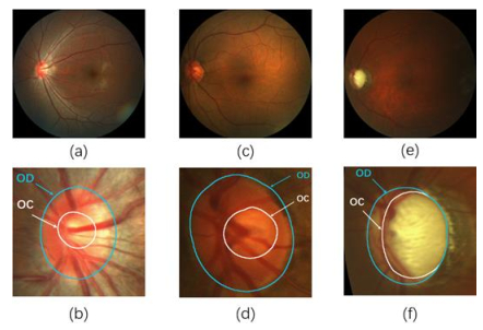
Glaucoma is a chronic neurodegenerative disease that can result in irreversible vision loss if not treated in its early stages. The cup-to-disc ratio is a key criterion for glaucoma screening and diagnosis, and it is determined by dividing the area of the optic cup (OC) by that of the optic disc (OD) in fundus images. Consequently, the automatic and accurate segmentation of the OC and OD is a pivotal step in glaucoma detection. In recent years, numerous methods have resulted in great success on this task. However, most existing methods either have unsatisfactory segmentation accuracy or high time costs. In this paper, we propose a lightweight deep-learning architecture for the simultaneous segmentation of the OC and OD, where we have adopted fuzzy learning and a multi-layer perceptron to simplify the learning complexity and improve segmentation accuracy. Experimental results demonstrate the superiority of our proposed method as compared to most state-of-the-art approaches in terms of both training time and segmentation accuracy.
- fuzzy learning,
- multi-layer perceptron,
- neural networks optic disc segmentation,
- optic cup segmentation,
- glaucoma screening
Citation: Yantao Song, Wenjie Zhang, Yue Zhang. A novel lightweight deep learning approach for simultaneous optic cup and optic disc segmentation in glaucoma detection[J]. Mathematical Biosciences and Engineering, 2024, 21(4): 5092-5117. doi: 10.3934/mbe.2024225

Related Papers:

Abstract

Glaucoma is a chronic neurodegenerative disease that can result in irreversible vision loss if not treated in its early stages. The cup-to-disc ratio is a key criterion for glaucoma screening and diagnosis, and it is determined by dividing the area of the optic cup (OC) by that of the optic disc (OD) in fundus images. Consequently, the automatic and accurate segmentation of the OC and OD is a pivotal step in glaucoma detection. In recent years, numerous methods have resulted in great success on this task. However, most existing methods either have unsatisfactory segmentation accuracy or high time costs. In this paper, we propose a lightweight deep-learning architecture for the simultaneous segmentation of the OC and OD, where we have adopted fuzzy learning and a multi-layer perceptron to simplify the learning complexity and improve segmentation accuracy. Experimental results demonstrate the superiority of our proposed method as compared to most state-of-the-art approaches in terms of both training time and segmentation accuracy.

References

[1]	V. S. Mary, E. B. Rajsingh, G. R. Naik, Retinal fundus image analysis for diagnosis of glaucoma: a comprehensive survey, IEEE Access, 4 (2016), 4327–4354. https://doi.org/10.1109/access.2016.2596761 doi: 10.1109/access.2016.2596761
[2]	Y. C. Tham, X. Li, T. Y. Wong, H. A. Quigley, T. Aung, C. Cheng, Global prevalence of glaucoma and projections of glaucoma burden through 2040: a systematic review and meta-analysis, Ophthalmology, 121 (2014), 2081–2090. https://doi.org/10.1016/j.ophtha.2014.05.013 doi: 10.1016/j.ophtha.2014.05.013
[3]	H. A. Quigley, A. T. Broman, The number of people with glaucoma worldwide in 2010 and 2020, Br J. ophthalmol., 90 (2006), 262–267. https://doi.org/10.1136/bjo.2005.081224 doi: 10.1136/bjo.2005.081224
[4]	M. U. Akram, A. Tariq, S. Khalid, M. Y. Javed, S. Abbas, U. U. Yasin, Glaucoma detection using novel optic disc localization, hybrid feature set and classification techniques, Australas. Phys. Eng. Sci. Med., 38 (2015), 643–655. https://doi.org/10.1007/s13246-015-0377-y doi: 10.1007/s13246-015-0377-y
[5]	M. A. Fernandez-Granero, A. Sarmiento, D. Sanchez-Morillo, S. Jiménez, P. Alemany, I. Fondón, Automatic CDR estimation for early glaucoma diagnosis, J. Healthc. Eng., 2017 (2017), 5953621. https://doi.org/10.1155/2017/5953621 doi: 10.1155/2017/5953621
[6]	S. Wang, L. Yu, X. Yang, C. W. Fu, P. A. Heng, Patch-based output space adversarial learning for joint optic disc and cup segmentation, IEEE Trans. Med. Imaging, 38 (2019), 2485–2495. https://doi.org/10.1109/TMI.2019.2899910 doi: 10.1109/TMI.2019.2899910
[7]	H. Fu, J. Cheng, Y. Xu, D. W. K. Wong, J. Liu, X. Cao, Joint optic disc and cup segmentation based on multi-label deep network and polar transformation, IEEE Trans. Med. Imaging, 37 (2018), 1597–1605. https://doi.org/10.1109/TMI.2018.2791488 doi: 10.1109/TMI.2018.2791488
[8]	Z. Zhang, H. Fu, H. Dai, J. Shen, Y. Pang, L. Shao, Et-net: A generic edge-attention guidance network for medical image segmentation, in Medical Image Computing and Computer Assisted Intervention, Springer International Publishing, (2019), 442. https://doi.org/10.1007/978-3-030-32239-7_49
[9]	S. Pathan, P. Kumar, R. Pai, S. V. Bhandary, Automated detection of optic disc contours in fundus images using decision tree classifier, Biocybern. Biomed. Eng., 40 (2020), 52–64. https://doi.org/10.1016/j.bbe.2019.11.003 doi: 10.1016/j.bbe.2019.11.003
[10]	P. S. Mittapalli, G. B. Kande, Segmentation of optic disk and optic cup from digital fundus images for the assessment of glaucoma, Biomed. Signal Process. Control, 24 (2016), 34–46. https://doi.org/10.1016/j.bspc.2015.09.003 doi: 10.1016/j.bspc.2015.09.003
[11]	D. W. K. Wong, J. Liu, J. H. Lim, X. Jia, F. Yin, H. Li, et al., Level-set based automatic cup-to-disc ratio determination using retinal fundus images in ARGALI, in 2008 30th annual international conference of the IEEE engineering in medicine and biology society, (2008), 2266. https://doi.org/10.1109/IEMBS.2008.4649648
[12]	J. Liu, D. W. K. Wong, J. H. Lim, X. Jia, F. Yin, H. Li, et al., Optic cup and disk extraction from retinal fundus images for determination of cup-to-disc ratio, in 2008 3rd IEEE Conference on Industrial Electronics and Applications, (2008), 1828. https://doi.org/10.1109/ICIEA.2008.4582835
[13]	R. A. Abdel-Ghafar, T. Morris, Progress towards automated detection and characterization of the optic disc in glaucoma and diabetic retinopathy, Med. Inform. Int. Med., 32 (2007), 19–25. https://doi.org/10.1080/14639230601095865 doi: 10.1080/14639230601095865
[14]	F. Mendels, C. Heneghan, J. Thiran, Identification of the optic disk boundary in retinal images using active contours, in Proceedings of Irish Machine Vision and Image Processing Conference (IMVIP), (1999), 103.
[15]	M. Lalonde, M. Beaulieu, L. Gagnon, Fast and robust optic disc detection using pyramidal decomposition and Hausdorff-based template matching, IEEE Trans. Med. Imaging, 20 (2001), 1193–1200. https://doi.org/10.1109/42.963823 doi: 10.1109/42.963823
[16]	S. Li, X. Sui, X. Luo, X. Xu, Y. Liu, R. Goh, Medical image segmentation using squeeze-and-expansion transformers, preprint, arXiv: 2105.09511.
[17]	J. Wu, H. Fang, F. Shang, D. Yang, Z. Wang, J. Gao, et al., SeATrans: learning segmentation-assisted diagnosis model via transformer, in International Conference on Medical Image Computing and Computer-Assisted Intervention, Springer Nature Switzerland, (2022), 677. https://doi.org/10.1007/978-3-031-16434-7_65
[18]	T. Yu, X. Li, Y. Cai, M. Sun, P. Li, S2-mlp: Spatial-shift mlp architecture for vision, in Proceedings of the IEEE/CVF winter conference on applications of computer vision, (2022), 297. https://doi.org/10.1109/WACV51458.2022.00367
[19]	D. Lian, Z. Yu, X. Sun, S. Gao, As-mlp: An axial shifted mlp architecture for vision, preprint, arXiv: 2107.08391. https://doi.org/10.48550/arXiv.2107.08391
[20]	I. O. Tolstikhin, N. Houlsby, A. Kolesnikov, L. Beyer, X. Zhai, T. Unterthiner, et al., Mlp-mixer: An all-mlp architecture for vision, Adv. Neural Inform. Process. Syst. 34 (2021), 24261–24272.
[21]	A. Dosovitskiy, L. Beyer, A. Kolesnikov, D. Weissenborn, X. Zhai, T. Unterthiner, et al., An image is worth 16x16 words: Transformers for image recognition at scale, preprint, arXiv: 2010.11929. https://doi.org/10.48550/arXiv.2010.11929
[22]	J. M. J. Valanarasu, V. M. Patel, UNeXt: MLP-based rapid medical image segmentation network, preprint, arXiv: 2203.04967. https://doi.org/10.48550/arXiv.2010.11929
[23]	H. K. Kwan, Y. Cai, A fuzzy neural network and its application to pattern recognition, IEEE Trans. Fuzzy Syst., 2 (1994), 185–193. https://doi.org/10.1109/91.298447 doi: 10.1109/91.298447
[24]	S. Zhou, Q. Chen, X. Wang, Fuzzy deep belief networks for semi-supervised sentiment classification, Neurocomputing, 131 (2014), 312–322. https://doi.org/10.1016/j.neucom.2013.10.011 doi: 10.1016/j.neucom.2013.10.011
[25]	R. Zhang, F. Shen, J. Zhao, A model with fuzzy granulation and deep belief networks for exchange rate forecasting, in 2014 international joint conference on neural networks (IJCNN), (2014), 366. https://doi.org/10.1109/IJCNN.2014.6889448
[26]	G. PadmaPriya, K. Duraiswamy, K. Rangasamy, Association of deep learning algorithm with fuzzy logic for multidocument text summarization, J. Theor. Appl. Inform. Technol., 62 (2014).
[27]	Sun. M, Huang. W, Wang. J. Density-Sorting-Based convolutional fuzzy min-max neural network for image classification, in 2021 International joint conference on neural networks (IJCNN), (2021), 1. https://doi.org/10.1109/IJCNN52387.2021.9534394
[28]	Y. Deng, Z. Ren, Y. Kong, F. Bao, Q. Dai, A hierarchical fused fuzzy deep neural network for data classification, IEEE Trans. Fuzzy Syst., 25 (2016), 1006–1012. https://doi.org/10.1109/TFUZZ.2016.2574915 doi: 10.1109/TFUZZ.2016.2574915
[29]	T. Shen, J. Wang, C. Gou, F. Y. Wang, Hierarchical fused model with deep learning and type-2 fuzzy learning for breast cancer diagnosis, IEEE Trans. Fuzzy Syst. 28 (2020), 3204–3218. https://doi.org/10.1109/TFUZZ.2020.3013681 doi: 10.1109/TFUZZ.2020.3013681
[30]	L. A. Zadeh, Fuzzy Sets, Inf. Control, (1965), 338–353. https://doi.org/10.1016/S0019-9958(65)90241-X doi: 10.1016/S0019-9958(65)90241-X
[31]	C. T. Lin, C. S. G. Lee, Neural-network-based fuzzy logic control and decision system, IEEE Trans. Comput., 40 (1991), 1320–1336. https://doi.org/10.1109/12.106218 doi: 10.1109/12.106218
[32]	J. J. Buckley, Y. Hayashi, Fuzzy neural networks: A survey, Fuzzy Sets Syst., 66 (1994), 1–13. https://doi.org/10.1016/0165-0114(94)90297-6 doi: 10.1016/0165-0114(94)90297-6
[33]	K. Hornik, M. Stinchcombe, H. White, Multilayer feedforward networks are universal approximators, Neural Networks, 2 (1989), 359–366. https://doi.org/10.1016/0893-6080(89)90020-8 doi: 10.1016/0893-6080(89)90020-8
[34]	M. Egmont-Petersen, D. de Ridder, H. Handels, Image processing with neural networks—a review, Pattern Recogn., 35 (2002), 2279–2301. https://doi.org/10.1016/S0031-3203(01)00178-9 doi: 10.1016/S0031-3203(01)00178-9
[35]	A. Krizhevsky, I. Sutskever, G. E. Hinton, Imagenet classification with deep convolutional neural networks, Adv. Neural Inform. Processing Syst., 25 (2012).
[36]	C. Farabet, C. Couprie, L. Najman, Y. LeCun, Learning hierarchical features for scene labeling, IEEE Trans. Pattern Anal. Mach. Intell., 35 (2012), 1915–1929. https://doi.org/1915-1929.10.1109/TPAMI.2012.231
[37]	Z. Yan, H. Zhang, B. Wang, S. Paris, Y. Yu, Automatic photo adjustment using deep neural networks, ACM Trans. Graph., 35 (2016), 1–15. https://doi.org/10.1145/2790296 doi: 10.1145/2790296
[38]	H. Greenspan, B. Van Ginneken, R. M. Summers, Guest editorial deep learning in medical imaging: Overview and future promise of an exciting new technique, IEEE Trans. Med. Imaging, 35 (2016), 1153–1159. https://doi.org/10.1109/TMI.2016.2553401 doi: 10.1109/TMI.2016.2553401
[39]	I. Yilmaz, Comparison of landslide susceptibility mapping methodologies for Koyulhisar, Turkey: conditional probability, logistic regression, artificial neural networks, and support vector machine, Environm. Earth Sci., 61 (2010), 821–836. https://doi.org/10.1007/s12665-009-0394-9 doi: 10.1007/s12665-009-0394-9
[40]	G. Z. M. Jalali, R. E. Nouri, Prediction of municipal solid waste generation by use of artificial neural network: A case study of Mashhad, Int. J. Environ. Res., 2 (2008), 13–22.
[41]	A. Howard, M. Sandler, G. Chu, L. C. Chen, B. Chen, M. Tan, et al., Searching for mobilenetv3, in Proceedings of the IEEE/CVF international conference on computer vision, (2019), 1314. https://doi.org/10.1109/ICCV.2019.00140
[42]	C. Cui, T. Gao, S. Wei, Y.Du, R. Guo, S. Dong, et al., PP-LCNet: A lightweight CPU convolutional neural network, preprint, arXiv: 2109.15099. https://doi.org/10.48550/arXiv.2109.15099
[43]	K. He, X. Zhang; S. Ren, J. Sun, Deep residual learning for image recognition, in Proceedings of the IEEE conference on computer vision and pattern recognition, (2016), 770. https://doi.org/10.1109/CVPR.2016.90
[44]	P. Ramachandran, B. Zoph, Q. V. Le, Searching for activation functions, preprint, arXiv: 1710.05941.
[45]	Z. Liu, Y. Lin, Y. Cao, H. Hu, Y. Wei, Z. Zhang, et al., Swin transformer: Hierarchical vision transformer using shifted windows, in Proceedings of the IEEE/CVF international conference on computer vision, (2021), 10012.
[46]	H. Zhao, J. Shi, X. Qi, X. Wang, J. Jia, Pyramid scene parsing network, in Proceedings of the IEEE conference on computer vision and pattern recognition, (2017), 2881. https://doi.org/10.1109/CVPR.2017.660
[47]	J. Sivaswamy, S. R. Krishnadas, G. D. Joshi, M. Jain, A. U. S. Tabish, Drishti-gs: Retinal image dataset for optic nerve head (onh) segmentation, in 2014 IEEE 11th international symposium on biomedical imaging (ISBI), (2014), 53. https://doi.org/10.1109/ISBI.2014.6867807
[48]	F. Fumero, S. Alayon, J. L. Sanchez, J. Sigut, M. Gonzalez-Hernandez, RIM-ONE: An open retinal image database for optic nerve evaluation, in 2011 24th international symposium on computer-based medical systems (CBMS), (2011), 1. https://doi.org/10.1109/CBMS.2011.5999143
[49]	J. I. Orlando, H. Fu, J. B. Breda, K. Van Keer, D. R. Bathula, A. Diaz-Pinto, et al., Refuge challenge: A unified framework for evaluating automated methods for glaucoma assessment from fundus photographs, Med. Image Anal., 59 (2020), 101570. https://doi.org/10.1016/j.media.2019.101570 doi: 10.1016/j.media.2019.101570
[50]	O. Ronneberger, P. Fischer, T. Brox, U-net: Convolutional networks for biomedical image segmentation, in Medical Image Computing and Computer-Assisted Intervention–MICCAI 2015: 18th International Conference, (2015), 234. https://doi.org/10.1007/978-3-319-24574-4_28
[51]	S. Wang, L. Yu, X. Yang, C. W. Fu, P. A. Heng, Patch-based output space adversarial learning for joint optic disc and cup segmentation, IEEE Trans. Med. Imaging, 38 (2019), 2485–2495. https://doi.org/10.1109/TMI.2019.2899910 doi: 10.1109/TMI.2019.2899910
[52]	H. Fu, J. Cheng, Y. Xu, D. W. K. Wong, J. Liu, X. Cao, Joint optic disc and cup segmentation based on multi-label deep network and polar transformation, IEEE Trans. Med. Imaging, 37 (2018), 1597–1605. https://doi.org/10.1109/TMI.2018.2791488 doi: 10.1109/TMI.2018.2791488
[53]	L. Luo, D. Xue, F. Pan, X. Feng, Joint optic disc and optic cup segmentation based on boundary prior and adversarial learning, Int. J. Comput. Assist. Radiol. Surgery, 16 (2021), 905–914. https://doi.org/10.1007/s11548-021-02373-6 doi: 10.1007/s11548-021-02373-6
[54]	Q. Zhu, X. Chen, Q. Meng, J. Song, G. Luo, M. Wang, et al., GDCSeg-Net: general optic disc and cup segmentation network for multi-device fundus images, Biomed. Optics Express, 12 (2021), 6529–6544. https://doi.org/10.1364/BOE.434841 doi: 10.1364/BOE.434841
[55]	R. Ali, B. Sheng, P. Li, Y. Chen, H. Li, P. Yang, et al., Optic disk and cup segmentation through fuzzy broad learning system for glaucoma screening, IEEE Trans. Industri. Inform., 17 (2020), 2476–2487. https://doi.org/10.1109/TII.2020.3000204 doi: 10.1109/TII.2020.3000204
[56]	Z. Gu, J. Cheng, H. Fu, K. Zhou, H. Hao, Y. Zhao, et al., Ce-net: Context encoder network for 2d medical image segmentation, IEEE Trans. Med. Imaging, 38 (2019), 2281–2292. https://doi.org/10.1109/TMI.2019.2903562 doi: 10.1109/TMI.2019.2903562
[57]	Z. Zhang, H. Fu, H. Dai, J. Shen, Y. Pang, L. Shao, Et-net: A generic edge-attention guidance network for medical image segmentation, in 22nd International Conference, Springer International Publishing, (2019), 442–450. https://doi.org/10.1007/978-3-030-32239-7_49
[58]	N. Ma, X. Zhang, H. T. Zheng, J. Sun, Shufflenet v2: Practical guidelines for efficient CNN architecture design, in Proceedings of the European conference on computer vision (ECCV), (2018), 116. https://doi.org/10.1007/978-3-030-01264-9_8

Reader Comments

Your name:*

Email:*
© 2024 the Author(s), licensee AIMS Press. This is an open access article distributed under the terms of the Creative Commons Attribution License (http://creativecommons.org/licenses/by/4.0)