SoftVoting6mA: An improved ensemble-based method for predicting DNA N6-methyladenine sites in cross-species genomes

Zhaoting Yin; Jianyi Lyu; Guiyang Zhang; Xiaohong Huang; Qinghua Ma; Jinyun Jiang; Zhaoting Yin; Jianyi Lyu; Guiyang Zhang; Xiaohong Huang; Qinghua Ma; Jinyun Jiang

doi:10.3934/mbe.2024169

Mathematical Biosciences and Engineering

2024, Volume 21, Issue 3: 3798-3815. doi: 10.3934/mbe.2024169

Previous Article Next Article

Research article

SoftVoting6mA: An improved ensemble-based method for predicting DNA N6-methyladenine sites in cross-species genomes

1.
College of Information Science and Engineering, Shaoyang University, Shaoyang 422000, China
2.
College of Information Science and Engineering, Hohai University, Nanjing 210000, China
3.
Faculty of Information Technology, University of Jyvaskyla, Jyvaskyla, Finland

Academic Editor: Danilo Pelusi

Received: 27 November 2023 Revised: 29 January 2024 Accepted: 05 February 2024 Published: 19 February 2024

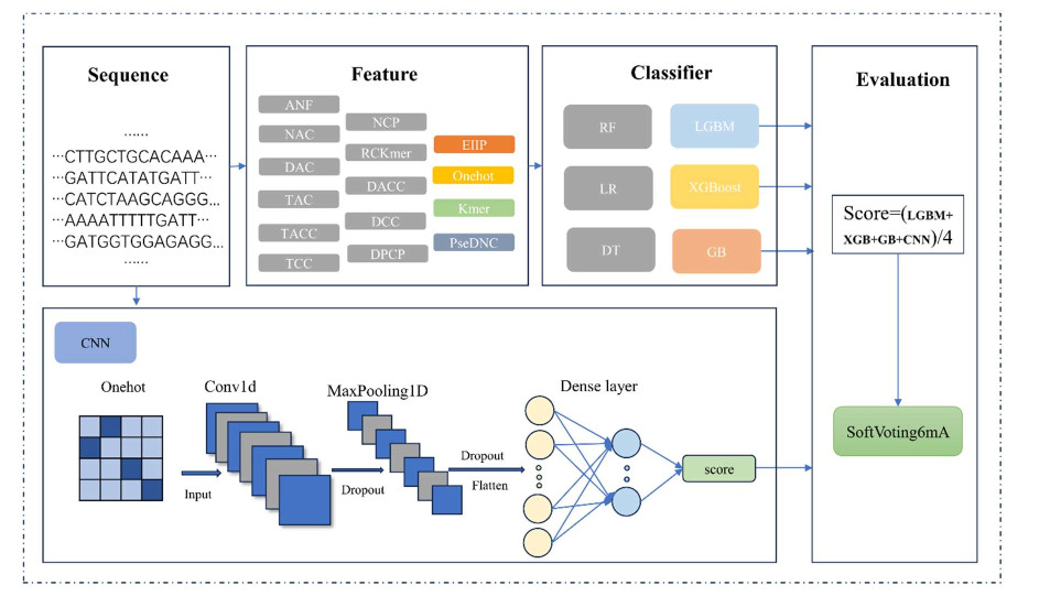
The DNA N6-methyladenine (6mA) is an epigenetic modification, which plays a pivotal role in biological processes encompassing gene expression, DNA replication, repair, and recombination. Therefore, the precise identification of 6mA sites is fundamental for better understanding its function, but challenging. We proposed an improved ensemble-based method for predicting DNA N6-methyladenine sites in cross-species genomes called SoftVoting6mA. The SoftVoting6mA selected four (electron–ion-interaction pseudo potential, One-hot encoding, Kmer, and pseudo dinucleotide composition) codes from 15 types of encoding to represent DNA sequences by comparing their performances. Similarly, the SoftVoting6mA combined four learning algorithms using the soft voting strategy. The 5-fold cross-validation and the independent tests showed that SoftVoting6mA reached the state-of-the-art performance. To enhance accessibility, a user-friendly web server is provided at http://www.biolscience.cn/SoftVoting6mA/.
- DNA N6-methyladenine,
- convolution neural network,
- soft voting,
- cross-species,
- feature fusion,
- webserver
Citation: Zhaoting Yin, Jianyi Lyu, Guiyang Zhang, Xiaohong Huang, Qinghua Ma, Jinyun Jiang. SoftVoting6mA: An improved ensemble-based method for predicting DNA N6-methyladenine sites in cross-species genomes[J]. Mathematical Biosciences and Engineering, 2024, 21(3): 3798-3815. doi: 10.3934/mbe.2024169

Related Papers:

Abstract

The DNA N6-methyladenine (6mA) is an epigenetic modification, which plays a pivotal role in biological processes encompassing gene expression, DNA replication, repair, and recombination. Therefore, the precise identification of 6mA sites is fundamental for better understanding its function, but challenging. We proposed an improved ensemble-based method for predicting DNA N6-methyladenine sites in cross-species genomes called SoftVoting6mA. The SoftVoting6mA selected four (electron–ion-interaction pseudo potential, One-hot encoding, Kmer, and pseudo dinucleotide composition) codes from 15 types of encoding to represent DNA sequences by comparing their performances. Similarly, the SoftVoting6mA combined four learning algorithms using the soft voting strategy. The 5-fold cross-validation and the independent tests showed that SoftVoting6mA reached the state-of-the-art performance. To enhance accessibility, a user-friendly web server is provided at http://www.biolscience.cn/SoftVoting6mA/.

References

[1]	V. R. Liyanage, J. S. Jarmasz, N. Murugeshan, M. R. Del Bigio, M. Rastegar, J. R. Davie, DNA Modifications: Function and Applications in Normal and Disease States, Biology, 3 (2014), 670–723. https://doi.org/10.3390/biology3040670 doi: 10.3390/biology3040670
[2]	S. Hiraoka, T. Sumida, M. Hirai, A. Toyoda, S. Kawagucci, T. Yokokawa, et al., Diverse DNA modification in marine prokaryotic and viral communities, Nucleic Acids Res., 50 (2022), 1531–1550. https://doi.org/10.1093/nar/gkab1292 doi: 10.1093/nar/gkab1292
[3]	H. Li, N. Zhang, Y. Wang, S. Xia, Y. Zhu, C. Xing, et al., DNA N6-Methyladenine Modification in Eukaryotic Genome, Front. Genet., 13 (2022), 914404. https://doi.org/10.3389/fgene.2022.914404 doi: 10.3389/fgene.2022.914404
[4]	C. L. Xiao, S. Zhu, M. He, D. Chen, Q. Zhang, Y. Chen, et al., N6-methyladenine DNA Modification in the Human Genome, Mol. Cell, 71 (2018), 306–318. e7. https://doi.org/10.1016/j.molcel.2018.06.015 doi: 10.1016/j.molcel.2018.06.015
[5]	E. L. Greer, M. A. Blanco, L. Gu, E. Sendinc, J. Liu, D. Aristizábal-Corrales, et al., DNA Methylation on N6-adenine in C. elegans, Cell, 161 (2015), 868–878. https://doi.org/10.1016/j.cell.2015.04.005 doi: 10.1016/j.cell.2015.04.005
[6]	C. Ma, R. Niu, T. Huang, L. W. Shao, Y. Peng, W. Ding, et al., N6-methyldeoxyadenine is a transgenerational epigenetic signal for mitochondrial stress adaptation, Nat. Cell Biol., 21 (2019), 319–327. https://doi.org/10.1038/s41556-018-0238-5 doi: 10.1038/s41556-018-0238-5
[7]	C. Zhou, C. Wang, H. Liu, Q. Zhou, Q. Liu, Y. Guo, et al., Identification and analysis of adenine N 6-methylation sites in the rice genome, Nat. Plants, 4 (2018), 554–563. https://doi.org/10.1038/s41477-018-0214-x doi: 10.1038/s41477-018-0214-x
[8]	J. Liu, Y. Zhu, G. Z. Luo, X. Wang, Y. Yue, X. Wang, et al., Abundant DNA 6mA methylation during early embryogenesis of zebrafish and pig, Nat. Commun., 7 (2016), 13052. https://doi.org/10.1038/ncomms13052 doi: 10.1038/ncomms13052
[9]	T. P. Wu, T. Wang, M. G. Seetin, Y. Lai, S. Zhu, K. Lin, et al., DNA methylation on N6-adenine in mammalian embryonic stem cells, Nature, 532 (2016), 329–333. https://doi.org/10.1038/nature17640 doi: 10.1038/nature17640
[10]	Z. K. O'Brown, E. L. Greer, N6-Methyladenine: A Conserved and Dynamic DNA Mark, DNA methyltransferases-role funct., 945 (2016), 213–246. https://doi.org/10.1007/978-3-319-43624-1_10 doi: 10.1007/978-3-319-43624-1_10
[11]	S. Lv, X. Zhou, Y. M. Li, T. Yang, S. J. Zhang, Y. Wang, et al., N6-methyladenine-modified DNA was decreased in Alzheimer's disease patients, World J. Clin. Cases, 10 (2022), 448–457. https://doi.org/10.12998/wjcc.v10.i2.448 doi: 10.12998/wjcc.v10.i2.448
[12]	Q. Lin, J. W. Chen, H. Yin, M. A. Li, C. R. Zhou, T. F. Hao, et al., DNA N6-methyladenine involvement and regulation of hepatocellular carcinoma development, Genomics, 114 (2022), 110265. https://doi.org/10.1016/j.ygeno.2022.01.002 doi: 10.1016/j.ygeno.2022.01.002
[13]	X. Sheng, J. Wang, Y. Guo, J. Zhang, J. Luo, DNA N6-Methyladenine (6mA) Modification Regulates Drug Resistance in Triple Negative Breast Cancer, Front. Oncol., 10 (2021), 616098. https://doi.org/10.3389/fonc.2020.616098 doi: 10.3389/fonc.2020.616098
[14]	S. Schiffers, C. Ebert, R. Rahimoff, O. Kosmatchev, J. Steinbacher, A.V. Bohne, et al., Quantitative LC–MS Provides No Evidence for m6dA or m4dC in the Genome of Mouse Embryonic Stem Cells and Tissues, Angew. Chem. Int. Ed., 56 (2017), 11268–11271. https://doi.org/10.1002/anie.201700424 doi: 10.1002/anie.201700424
[15]	K. Han, J. Wang, Y. Wang, L. Zhang, M. Yu, F. Xie, et al., A review of methods for predicting DNA N6-methyladenine sites, Briefings Bioinf., 24 (2023), bbac514. https://doi.org/10.1093/bib/bbac514 doi: 10.1093/bib/bbac514
[16]	H. Xu, R. Hu, P. Jia, Z. J. B. Zhao, 6mA-Finder: a novel online tool for predicting DNA N6-methyladenine sites in genomes, Bioinformatics, 36 (2020), 3257–3259. https://doi.org/10.1093/bioinformatics/btaa113 doi: 10.1093/bioinformatics/btaa113
[17]	H. Yu, Z. Dai, SNNRice6mA: A Deep Learning Method for Predicting DNA N6-Methyladenine Sites in Rice Genome, Front. Genet., 10 (2019), 1071. https://doi.org/10.3389/fgene.2019.01071 doi: 10.3389/fgene.2019.01071
[18]	M. Tahir, H. Tayara, K. T. Chong, iDNA6mA (5-step rule): Identification of DNA N6-methyladenine sites in the rice genome by intelligent computational model via Chou's 5-step rule, Chemom. Intell. Lab. Syst., 189 (2019), 96–101. https://doi.org/10.1016/j.chemolab.2019.04.007 doi: 10.1016/j.chemolab.2019.04.007
[19]	X. Tang, P. Zheng, X. Li, H. Wu, D. Q. Wei, Y. Liu, et al., Deep6mAPred: A CNN and Bi-LSTM-based deep learning method for predicting DNA N6-methyladenosine sites across plant species, Methods, 204 (2022), 142–150. https://doi.org/10.1016/j.ymeth.2022.04.011 doi: 10.1016/j.ymeth.2022.04.011
[20]	M.M. Hasan, B. Manavalan, W. Shoombuatong, M. S. Khatun, H. Kurata, i6mA-Fuse: improved and robust prediction of DNA 6 mA sites in the Rosaceae genome by fusing multiple feature representation, Plant Mol. Biol., 103 (2020), 225–234. https://doi.org/10.1007/s11103-020-00988-y doi: 10.1007/s11103-020-00988-y
[21]	Z. Abbas, M. ur Rehman, H. Tayara, Q. Zou, K. T. Chong, XGBoost framework with feature selection for the prediction of RNA N5-methylcytosine sites, Mol. Ther., 2023. https://doi.org/10.1016/j.ymthe.2023.05.016 doi: 10.1016/j.ymthe.2023.05.016
[22]	P. Feng, H. Yang, H. Ding, H. Lin, W. Chen, K. C. Chou, iDNA6mA-PseKNC: Identifying DNA N6-methyladenosine sites by incorporating nucleotide physicochemical properties into PseKNC, Genomics, 111 (2019), 96–102. https://doi.org/10.1016/j.ygeno.2018.01.005 doi: 10.1016/j.ygeno.2018.01.005
[23]	H. Lv, F. Y. Dao, Z. X. Guan, D. Zhang, J. X. Tan, Y. Zhang, et al., iDNA6mA-Rice: A Computational Tool for Detecting N6-Methyladenine Sites in Rice, Front. Genet., 10 (2019), 793. https://doi.org/10.3389/fgene.2019.00793 doi: 10.3389/fgene.2019.00793
[24]	Q. Huang, J. Zhang, L. Wei, F. Guo, Q. Zou, 6mA-RicePred: A Method for Identifying DNA N6-Methyladenine Sites in the Rice Genome Based on Feature Fusion, Front. Plant Sci., 11 (2020), 4. https://doi.org/10.3389/fpls.2020.00004 doi: 10.3389/fpls.2020.00004
[25]	Z. Teng, Z. Zhao, Y. Li, Z. Tian, M. Guo, Q. Lu, et al., i6mA-Vote: Cross-Species Identification of DNA N6-Methyladenine Sites in Plant Genomes Based on Ensemble Learning With Voting, Front. Plant Sci., 13 (2022), 845835. https://doi.org/10.3389/fpls.2022.845835 doi: 10.3389/fpls.2022.845835
[26]	J. Khanal, D. Y. Lim, H. Tayara, K. T. Chong, i6mA-stack: A stacking ensemble-based computational prediction of DNA N6-methyladenine (6mA) sites in the Rosaceae genome, Genomics, 113 (2021), 582–592. https://doi.org/10.1016/j.ygeno.2020.09.054 doi: 10.1016/j.ygeno.2020.09.054
[27]	Z. Abbas, H. Tayara, K. to Chong, SpineNet-6mA: A Novel Deep Learning Tool for Predicting DNA N6-Methyladenine Sites in Genomes, IEEE Access, 8 (2020), 201450–201457. https://doi.org/10.1109/ACCESS.2020.3036090
[28]	A. Wahab, S. D. Ali, H. Tayara, K. T. Chong, iIM-CNN: Intelligent Identifier of 6mA Sites on Different Species by Using Convolution Neural Network, IEEE Access, 7 (2019), 178577–178583. https://doi.org/10.1109/ACCESS.2019.2958618 doi: 10.1109/ACCESS.2019.2958618
[29]	C. R. Rahman, R. Amin, S. Shatabda, M. S. I. Toaha, A convolution based computational approach towards DNA N6-methyladenine site identification and motif extraction in rice genome, Sci. Rep., 11 (2021), 10357. https://doi.org/10.1038/s41598-021-89850-9 doi: 10.1038/s41598-021-89850-9
[30]	Z. Li, H. Jiang, L. Kong, Y. Chen, K. Lang, X. Fan, et al., Deep6mA: a deep learning framework for exploring similar patterns in DNA N6-methyladenine sites across different species, PLoS Comput. Biol., 17 (2021), e1008767. https://doi.org/10.1371/journal.pcbi.1008767 doi: 10.1371/journal.pcbi.1008767
[31]	N. Q. K. Le, Q. T. Ho, Deep transformers and convolutional neural network in identifying DNA N6-methyladenine sites in cross-species genomes, Methods, 204 (2022), 199–206. https://doi.org/10.1016/j.ymeth.2021.12.004 doi: 10.1016/j.ymeth.2021.12.004
[32]	W. Bao, Q. Cui, B. Chen, B. Yang, Phage_UniR_LGBM: phage virion proteins classification with UniRep features and LightGBM model, Comput. math. methods med., 2022 (2022). https://doi.org/10.1155/2022/9470683 doi: 10.1155/2022/9470683
[33]	W. Bao, Y. Gu, B. Chen, H. Yu, Golgi_DF: Golgi proteins classification with deep forest, Front. Neurosci., 17 (2023), 1197824. https://doi.org/10.3389/fnins.2023.1197824 doi: 10.3389/fnins.2023.1197824
[34]	W. Bao, B. Yang, B. Chen, 2-hydr_ensemble: lysine 2-hydroxyisobutyrylation identification with ensemble method, Chemom. Intell. Lab. Syst., 215 (2021), 104351. https://doi.org/10.1016/j.chemolab.2021.104351 doi: 10.1016/j.chemolab.2021.104351
[35]	P. Ye, Y. Luan, K. Chen, Y. Liu, C. Xiao, Z. Xie, MethSMRT: an integrative database for DNA N6-methyladenine and N4-methylcytosine generated by single-molecular real-time sequencing, Nucleic Acids Res., 45 (2016), D85–D89. https://doi.org/10.1093/nar/gkw950 doi: 10.1093/nar/gkw950
[36]	W. Chen, H. Lv, F. Nie, H. Lin, i6mA-Pred: identifying DNA N6-methyladenine sites in the rice genome, Bioinformatics, 35 (2019), 2796–2800. https://doi.org/10.1093/bioinformatics/btz015 doi: 10.1093/bioinformatics/btz015
[37]	L. Fu, B. Niu, Z. Zhu, S. Wu, W. J. B. Li, CD-HIT: accelerated for clustering the next-generation sequencing data, Bioinformatics, 28 (2012), 3150–3152. https://doi.org/10.1093/bioinformatics/bts565 doi: 10.1093/bioinformatics/bts565
[38]	G. Ke, Q. Meng, T. Finley, T. Wang, W. Chen, W. Ma, et al., Lightgbm: A highly efficient gradient boosting decision tree, Adv. neural inf. process. syst., 30 (2017), 3149–3157. https://dl.acm.org/doi/10.5555/3294996.3295074
[39]	T. Chen, C. Guestrin, Xgboost: A scalable tree boosting system, in Proceedings of the 22nd Acm Sigkdd International Conference on Knowledge Discovery and Data Mining, Association for Computing Machinery, New York, (2016), 785–794. https://doi.org/10.1145/2939672.2939785
[40]	A. Natekin, A. Knoll, Gradient boosting machines, a tutorial, Front. Neurorob., 7 (2013), 21. https://doi.org/10.3389/fnbot.2013.00021 doi: 10.3389/fnbot.2013.00021
[41]	M. Pal, Random forest classifier for remote sensing classification, Int. J. Remote Sens., 26 (2005), 217–222. https://doi.org/10.1080/01431160412331269698 doi: 10.1080/01431160412331269698
[42]	L. G. Grimm, P. R. Yarnold, Reading and Understanding Multivariate Statistics, American Psychological Association, Washington, 1995. https://doi.org/10.1152/advan.00006.2004
[43]	S. R. Safavian, D. Landgrebe, A survey of decision tree classifier methodology, IEEE Trans. Syst. Man Cybern., 21 (1991), 660–674. https://doi.org/10.1109/21.97458 doi: 10.1109/21.97458
[44]	J. Inglesfield, A method of embedding, J. Phys. C: Solid State Phys., 14 (1981), 3795. https://doi.org/10.1088/0022-3719/14/26/015 doi: 10.1088/0022-3719/14/26/015
[45]	S. Albawi, T. A. Mohammed, S. Al-Zawi, Understanding of a convolutional neural network, in 2017 International Conference on Engineering and Technology (ICET), Akdeniz University, Antalya, (2017), 1–6. https://doi.org/10.1109/ICEngTechnol.2017.8308186
[46]	D. Lalović, V. Veljković, The global average DNA base composition of coding regions may be determined by the electron-ion interaction potential, Biosystems, 23 (1990), 311–316. https://doi.org/10.1016/0303-2647(90)90013-Q doi: 10.1016/0303-2647(90)90013-Q
[47]	W. He, C. Jia, EnhancerPred2. 0: predicting enhancers and their strength based on position-specific trinucleotide propensity and electron–ion interaction potential feature selection, Mol. Biosyst., 13 (2017), 767–774. https://doi.org/10.1039/C7MB00054E doi: 10.1039/C7MB00054E
[48]	W. He, C. Jia, Q. Zou, 4mCPred: machine learning methods for DNA N4-methylcytosine sites prediction, Bioinformatics, 35 (2019), 593–601. https://doi.org/10.1093/bioinformatics/bty668 doi: 10.1093/bioinformatics/bty668
[49]	P. Rodríguez, M.A. Bautista, J. Gonzalez, S. Escalera, Beyond one-hot encoding: lower dimensional target embedding, Image Vision Comput., 75 (2018), 21–31. https://doi.org/10.1016/j.imavis.2018.04.004 doi: 10.1016/j.imavis.2018.04.004
[50]	K. C. Chou, Prediction of protein cellular attributes using pseudo‐amino acid composition, Proteins Struct. Funct. Bioinf., 43 (2001), 246–255. https://doi.org/10.1002/prot.1035 doi: 10.1002/prot.1035
[51]	W. Chen, P. M. Feng, H. Lin, K. C. Chou, iRSpot-PseDNC: Identify recombination spots with pseudo dinucleotide composition, Nucleic Acids Res., 41 (2013), e68. https://doi.org/10.1093/nar/gks1450 doi: 10.1093/nar/gks1450
[52]	W. Chen, P. M. Feng, H. Lin, K. C. Chou, iSS-PseDNC: Identifying splicing sites using pseudo dinucleotide composition, Biomed Res. Int., 2014 (2014). https://doi.org/10.1155/2014/623149 doi: 10.1155/2014/623149
[53]	W. Chen, H. Ding, X. Zhou, H. Lin, K. C. Chou, iRNA(m6A)-PseDNC: identifying N6-methyladenosine sites using pseudo dinucleotide composition, Anal. Biochem., 561 (2018), 59–65. https://doi.org/10.1016/j.ab.2018.09.002 doi: 10.1016/j.ab.2018.09.002
[54]	Z. Cui, S. G. Wang, Y. He, Z. H. Chen, Q. H. Zhang, DeepTPpred: A deep learning approach with matrix factorization for predicting therapeutic peptides by integrating length information, IEEE J. Biomed. Health. Inf., 27 (2023), 4611–4622. https://doi.org/10.1109/jbhi.2023.3290014 doi: 10.1109/jbhi.2023.3290014
[55]	Z. Chen, P. Zhao, C. Li, F. Li, D. Xiang, Y. Z. Chen, et al., iLearnPlus: a comprehensive and automated machine-learning platform for nucleic acid and protein sequence analysis, prediction and visualization, Nucleic Acids Res., 49 (2021), e60. https://doi.org/10.1093/nar/gkab122 doi: 10.1093/nar/gkab122
[56]	Z. Liu, W. Dong, W. Jiang, Z. He, csDMA: an improved bioinformatics tool for identifying DNA 6 mA modifications via Chou's 5-step rule, Sci. Rep., 9 (2019), 13109. https://doi.org/10.1038/s41598-019-49430-4 doi: 10.1038/s41598-019-49430-4
[57]	M. M. Hasan, S. Basith, M. S. Khatun, G. Lee, B. Manavalan, H. Kurata, Meta-i6mA: an interspecies predictor for identifying DNA N 6-methyladenine sites of plant genomes by exploiting informative features in an integrative machine-learning framework, Briefings Bioinf., 22 (2021), bbaa202. https://doi.org/10.1093/bib/bbaa202 doi: 10.1093/bib/bbaa202
[58]	Z. Abbas, H. Tayara, K. T. Chong, ZayyuNet–A unified deep learning model for the identification of epigenetic modifications using raw genomic sequences, IEEE/ACM Trans. Comput. Biol. Bioinf., 19 (2021), 2533–2544. https://doi.org/10.1109/tcbb.2021.3083789 doi: 10.1109/tcbb.2021.3083789

mbe-21-03-169-supplementary.pdf

Reader Comments

Your name:*

Email:*
© 2024 the Author(s), licensee AIMS Press. This is an open access article distributed under the terms of the Creative Commons Attribution License (http://creativecommons.org/licenses/by/4.0)