In this paper, we introduce a novel deep learning method for dental panoramic image segmentation, which is crucial in oral medicine and orthodontics for accurate diagnosis and treatment planning. Traditional methods often fail to effectively combine global and local context, and struggle with unlabeled data, limiting performance in varied clinical settings. We address these issues with an advanced TransUNet architecture, enhancing feature retention and utilization by connecting the input and output layers directly. Our architecture further employs spatial and channel attention mechanisms in the decoder segments for targeted region focus, and deep supervision techniques to overcome the vanishing gradient problem for more efficient training. Additionally, our network includes a self-learning algorithm using unlabeled data, boosting generalization capabilities. Named the Semi-supervised Tooth Segmentation Transformer U-Net (STS-TransUNet), our method demonstrated superior performance on the MICCAI STS-2D dataset, proving its effectiveness and robustness in tooth segmentation tasks.
Citation: Duolin Sun, Jianqing Wang, Zhaoyu Zuo, Yixiong Jia, Yimou Wang. STS-TransUNet: Semi-supervised Tooth Segmentation Transformer U-Net for dental panoramic image[J]. Mathematical Biosciences and Engineering, 2024, 21(2): 2366-2384. doi: 10.3934/mbe.2024104
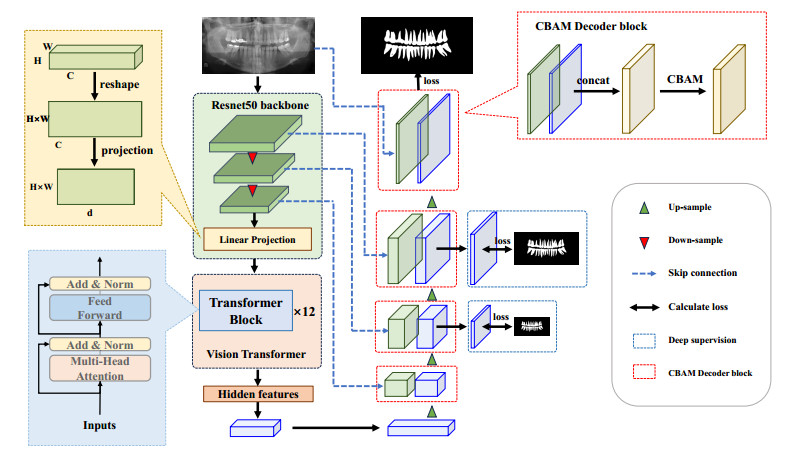
In this paper, we introduce a novel deep learning method for dental panoramic image segmentation, which is crucial in oral medicine and orthodontics for accurate diagnosis and treatment planning. Traditional methods often fail to effectively combine global and local context, and struggle with unlabeled data, limiting performance in varied clinical settings. We address these issues with an advanced TransUNet architecture, enhancing feature retention and utilization by connecting the input and output layers directly. Our architecture further employs spatial and channel attention mechanisms in the decoder segments for targeted region focus, and deep supervision techniques to overcome the vanishing gradient problem for more efficient training. Additionally, our network includes a self-learning algorithm using unlabeled data, boosting generalization capabilities. Named the Semi-supervised Tooth Segmentation Transformer U-Net (STS-TransUNet), our method demonstrated superior performance on the MICCAI STS-2D dataset, proving its effectiveness and robustness in tooth segmentation tasks.

| [1] |
P. Sanchez, B. Everett, Y. Salamonson, S. Ajwani, S. Bhole, J. Bishop, et al., Oral health and cardiovascular care: Perceptions of people with cardiovascular disease, PLoS One, 12 (2017), e0181189. https://doi.org/10.1371/journal.pone.0181189 doi: 10.1371/journal.pone.0181189

|
| [2] | M. P. Muresan, A. R. Barbura, S. Nedevschi, Teeth detection and dental problem classification in panoramic x-ray images using deep learning and image processing techniques, in 2020 IEEE 16th International Conference on Intelligent Computer Communication and Processing (ICCP), IEEE, (2020), 457–463. https://doi.org/10.1109/ICCP51029.2020.9266244 |
| [3] |
V. Hingst, M. A. Weber, Dental X-ray diagnostics with the orthopantomography–technique and typical imaging results, Der Radiologe, 60 (2020), 77–92. https://doi.org/10.1007/s00117-019-00620-1 doi: 10.1007/s00117-019-00620-1
|
| [4] |
J. C. M. Román, V. R. Fretes, C. G. Adorno, R. G. Silva, J. L. V. Noguera, H. Legal-Ayala, et al., Panoramic dental radiography image enhancement using multiscale mathematical morphology, Sensors, 21 (2021), 3110. https://doi.org/10.3390/s21093110 doi: 10.3390/s21093110
|
| [5] |
R. Izzetti, M. Nisi, G. Aringhieri, L. Crocetti, F. Graziani, C. Nardi, Basic knowledge and new advances in panoramic radiography imaging techniques: A narrative review on what dentists and radiologists should know, Appl. Sci., 11 (2021), 7858. https://doi.org/10.3390/app11177858 doi: 10.3390/app11177858
|
| [6] |
Y. Zhao, P. Li, C. Gao, Y. Liu, Q. Chen, F. Yang, et al., Tsasnet: Tooth segmentation on dental panoramic X-ray images by Two-Stage Attention Segmentation Network, Knowledge-Based Syst., 206 (2020), 106338. https://doi.org/10.1016/j.knosys.2020.106338 doi: 10.1016/j.knosys.2020.106338
|
| [7] |
A. E. Yüksel, S. Gültekin, E. Simsar, Ş. D. Özdemir, M. Gündoğar, S. B. Tokgöz, et al., Dental enumeration and multiple treatment detection on panoramic X-rays using deep learning, Sci. Rep., 11 (2021), 12342. https://doi.org/10.1038/s41598-021-90386-1 doi: 10.1038/s41598-021-90386-1
|
| [8] |
R. J. Lee, A. Weissheimer, J. Pham, L. Go, L. M. de Menezes, W. R. Redmond, et al., Three-dimensional monitoring of root movement during orthodontic treatment, Am. J. Orthod. Dentofacial Orthop., 147 (2015), 132–142. https://doi.org/10.1016/j.ajodo.2014.10.010 doi: 10.1016/j.ajodo.2014.10.010
|
| [9] | J. Keustermans, D. Vandermeulen, P. Suetens, Integrating statistical shape models into a graph cut framework for tooth segmentation, in Machine Learning in Medical Imaging, Springer, (2012), 242–249. https://doi.org/10.1007/978-3-642-35428-1_30 |
| [10] | O. Ronneberger, P. Fischer, T. Brox, U-Net: Convolutional networks for biomedical image segmentation, in Medical Image Computing and Computer-Assisted Intervention–MICCAI 2015, Springer, (2015), 234–241. https://doi.org/10.1007/978-3-319-24574-4_28 |
| [11] |
W. Wang, X. Yu, B. Fang, Y. Zhao, Y. Chen, W. Wei, et al., Cross-modality LGE-CMR segmentation using image-to-image translation based data augmentation, IEEE/ACM Trans. Comput. Biol. Bioinf., 20 (2023), 2367–2375. https://doi.org/10.1109/tcbb.2022.3140306 doi: 10.1109/tcbb.2022.3140306
|
| [12] |
W. Wang, J. Chen, J. Wang, J. Chen, J. Liu, Z. Gong, Trust-enhanced collaborative filtering for personalized point of interests recommendation, IEEE Trans. Ind. Inf., 16 (2020), 6124–6132. https://doi.org/10.1109/tii.2019.2958696 doi: 10.1109/tii.2019.2958696
|
| [13] |
B. G. He, B. Lin, H. P. Li, S. Q. Zhu, Suggested method of utilizing soil arching for optimizing the design of strutted excavations, Tunnelling Underground Space Technol., 143 (2024), 105450. https://doi.org/10.1016/j.tust.2023.105450 doi: 10.1016/j.tust.2023.105450
|
| [14] |
J. Chen, S. Sun, L. Zhang, B. Yang, W. Wang, Compressed sensing framework for heart sound acquisition in internet of medical things, IEEE Trans. Ind. Inf., 18 (2022), 2000–2009. https://doi.org/10.1109/tii.2021.3088465 doi: 10.1109/tii.2021.3088465
|
| [15] |
J. Chen, W. Wang, B. Fang, Y. Liu, K. Yu, V. C. M. Leung, et al., Digital twin empowered wireless healthcare monitoring for smart home, IEEE J. Sel. Areas Commun., 41 (2023), 3662–3676. https://doi.org/10.1109/jsac.2023.3310097 doi: 10.1109/jsac.2023.3310097
|
| [16] |
Y. Zhang, X. Wu, S. Lu, H. Wang, P. Phillips, S. Wang, Smart detection on abnormal breasts in digital mammography based on contrast-limited adaptive histogram equalization and chaotic adaptive real-coded biogeography-based optimization, Simulation, 92 (2016), 873–885. https://doi.org/10.1177/0037549716667834 doi: 10.1177/0037549716667834
|
| [17] |
J. H. Lee, S. S. Han, Y. H. Kim, C. Lee, I. Kim, Application of a fully deep convolutional neural network to the automation of tooth segmentation on panoramic radiographs, Oral Surg. Oral Med. Oral Pathol. Oral Radiol., 129 (2020), 635–642. https://doi.org/10.1016/j.oooo.2019.11.007 doi: 10.1016/j.oooo.2019.11.007
|
| [18] |
J. Chen, Z. Guo, X. Xu, L. Zhang, Y. Teng, Y. Chen, et al., A robust deep learning framework based on spectrograms for heart sound classification, IEEE/ACM Trans. Comput. Biol. Bioinf., 2023 (2023), 1–12. https://doi.org/10.1109/TCBB.2023.3247433 doi: 10.1109/TCBB.2023.3247433
|
| [19] |
S. H. Wang, D. R. Nayak, D. S. Guttery, X. Zhang, Y. D. Zhang, COVID-19 classification by CCSHNet with deep fusion using transfer learning and discriminant correlation analysis, Inf. Fusion, 68 (2021), 131–148. https://doi.org/10.1016/j.inffus.2020.11.005 doi: 10.1016/j.inffus.2020.11.005
|
| [20] | H. Chen, X. Huang, Q. Li, J. Wang, B. Fang, J. Chen, Labanet: Lead-assisting backbone attention network for oral multi-pathology segmentation, in ICASSP 2023-2023 IEEE International Conference on Acoustics, Speech and Signal Processing (ICASSP), IEEE, (2023), 1–5. https://doi.org/10.1109/ICASSP49357.2023.10094785 |
| [21] |
L. Wang, Y. Gao, F. Shi, G. Li, K. C. Chen, Z. Tang, et al., Automated segmentation of dental cbct image with prior-guided sequential random forests, Med. Phys., 43 (2016), 336–346. https://doi.org/10.1118/1.4938267 doi: 10.1118/1.4938267
|
| [22] |
S. Liao, S. Liu, B. Zou, X. Ding, Y. Liang, J. Huang, et al., Automatic tooth segmentation of dental mesh based on harmonic fields, Biomed Res. Int., 2015 (2015). https://doi.org/10.1155/2015/187173 doi: 10.1155/2015/187173
|
| [23] | R. Girshick, Fast R-CNN, in Proceedings of the IEEE International Conference on Computer Vision, (2015), 1440–1448. https://doi.org/10.1109/ICCV.2015.169 |
| [24] | K. He, G. Gkioxari, P. Dollár, R. Girshick, Mask R-CNN, in Proceedings of the IEEE International Conference on Computer Vision, (2017), 2961–2969. https://doi.org/10.1109/ICCV.2017.322 |
| [25] |
E. Y. Park, H. Cho, S. Kang, S. Jeong, E. Kim, Caries detection with tooth surface segmentation on intraoral photographic images using deep learning, BMC Oral Health, 22 (2022), 1–9. https://doi.org/10.1186/s12903-022-02589-1 doi: 10.1186/s12903-022-02589-1
|
| [26] | G. Zhu, Z. Piao, S. C. Kim, Tooth detection and segmentation with mask R-CNN, in 2020 International Conference on Artificial Intelligence in Information and Communication (ICAIIC), IEEE, (2020), 070–072. https://doi.org/10.1109/ICAIIC48513.2020.9065216 |
| [27] |
Q. Chen, Y. Zhao, Y. Liu, Y. Sun, C. Yang, P. Li, et al., Mslpnet: Multi-scale location perception network for dental panoramic X-ray image segmentation, Neural Comput. Appl., 33 (2021), 10277–10291. https://doi.org/10.1007/s00521-021-05790-5 doi: 10.1007/s00521-021-05790-5
|
| [28] |
P. Li, Y. Liu, Z. Cui, F. Yang, Y. Zhao, C. Lian, et al., Semantic graph attention with explicit anatomical association modeling for tooth segmentation from CBCT images, IEEE Trans. Med. Imaging, 41 (2022), 3116–3127. https://doi.org/10.1109/tmi.2022.3179128 doi: 10.1109/tmi.2022.3179128
|
| [29] |
E. Shaheen, A. Leite, K. A. Alqahtani, A. Smolders, A. Van Gerven, H. Willems, et al., A novel deep learning system for multi-class tooth segmentation and classification on Cone Beam Computed Tomography. A validation study, J. Dent., 115 (2021), 103865. https://doi.org/10.1016/j.jdent.2021.103865 doi: 10.1016/j.jdent.2021.103865
|
| [30] | M. Ezhov, A. Zakirov, M. Gusarev, Coarse-to-fine volumetric segmentation of teeth in cone-beam CT, in 2019 IEEE 16th International Symposium on Biomedical Imaging (ISBI 2019), (2019), 52–56. https://doi.org/10.1109/ISBI.2019.8759310 |
| [31] | A. Alsheghri, F. Ghadiri, Y. Zhang, O. Lessard, J. Keren, F. Cheriet, et al., Semi-supervised segmentation of tooth from 3D scanned dental arches, in Medical Imaging 2022: Image Processing, (2022), 766–771. https://doi.org/10.1117/12.2612655 |
| [32] |
X. Liu, F. Zhang, Z. Hou, L. Mian, Z. Wang, J. Zhang, et al., Self-supervised learning: Generative or contrastive, IEEE Trans. Knowl. Data Eng., 35 (2021), 857–876. https://doi.org/10.1109/tkde.2021.3090866 doi: 10.1109/tkde.2021.3090866
|
| [33] | Q. Li, X. Huang, Z. Wan, L. Hu, S. Wu, J. Zhang, et al., Data-efficient masked video modeling for self-supervised action recognition, in Proceedings of the 31st ACM International Conference on Multimedia, (2023), 2723–2733. https://doi.org/10.1145/3581783.3612496 |
| [34] |
H. Lim, S. Jung, S. Kim, Y. Cho, I. Song, Deep semi-supervised learning for automatic segmentation of inferior alveolar nerve using a convolutional neural network, BMC Oral Health, 21 (2021), 1–9. https://doi.org/10.2196/preprints.32088 doi: 10.2196/preprints.32088
|
| [35] |
F. Isensee, P. F. Jaeger, S. A. Kohl, J. Petersen, K. H. Maier-Hein, nnU-Net: A self-configuring method for deep learning-based biomedical image segmentation, Nat. Methods, 18 (2021), 203–211. https://doi.org/10.1038/s41592-020-01008-z doi: 10.1038/s41592-020-01008-z
|
| [36] | A. Dosovitskiy, L. Beyer, A. Kolesnikov, D. Weissenborn, X. Zhai, T. Unterthiner, et al., An image is worth 16x16 words: Transformers for image recognition at scale, arXiv preprint, (2020), arXiv: 2010.11929. https://doi.org/10.48550/arXiv.2010.11929 |
| [37] | H. Touvron, M. Cord, M. Douze, F. Massa, A. Sablayrolles, H. Jégou, Training data-efficient image transformers & distillation through attention, in International Conference on Machine Learning, PMLR, (2021), 10347–10357. |
| [38] | N. Carion, F. Massa, G. Synnaeve, N. Usunier, A. Kirillov, S. Zagoruyko, End-to-end object detection with transformers, in European Conference on Computer Vision, Springer, (2020), 213–229. https://doi.org/10.1007/978-3-030-58452-8_13 |
| [39] | X. Zhu, W. Su, L. Lu, B. Li, X. Wang, J. Dai, Deformable DETR: Deformable transformers for end-to-end object detection, arXiv preprint, (2020), arXiv: 2010.04159. https://doi.org/10.48550/arXiv.2010.04159 |
| [40] |
Q. Li, X. Huang, B. Fang, H. Chen, S. Ding, X. Liu, Embracing large natural data: Enhancing medical image analysis via cross-domain fine-tuning, IEEE J. Biomed. Health. Inf., 2023 (2023), 1–10. https://doi.org/10.1109/JBHI.2023.3343518 doi: 10.1109/JBHI.2023.3343518
|
| [41] | J. Chen, Y. Lu, Q. Yu, X. Luo, E. Adeli, Y. Wang, et al., Transunet: Transformers make strong encoders for medical image segmentation, arXiv preprint, arXiv: 2102.04306. https://doi.org/10.48550/arXiv.2102.04306 |
| [42] | A. Srinivas, T. Lin, N. Parmar, J. Shlens, P. Abbeel, A. Vaswani, Bottleneck transformers for visual recognition, in Proceedings of the IEEE/CVF Conference on Computer Vision and Pattern Recognition, (2021), 16519–16529. https://doi.org/10.1109/CVPR46437.2021.01625 |
| [43] | Y. Li, S. Wang, J. Wang, G. Zeng, W. Liu, Q. Zhang, et al., GT U-Net: A U-Net like group transformer network for tooth root segmentation, in Machine Learning in Medical Imaging, Springer, (2021), 386–395. https://doi.org/10.1007/978-3-030-87589-3_40 |
| [44] | W. Lin, Z. Wu, J. Chen, J. Huang, L. Jin, Scale-aware modulation meet transformer, arXiv preprint, (2023), arXiv: 2307.08579. https://doi.org/10.48550/arXiv.2307.08579 |
| [45] | S. Woo, J. Park, J. Lee, I. Kweon, CBAM: Convolutional block attention module, in Computer Vision–ECCV 2018, Springer, (2018), 3–19. https://doi.org/10.1007/978-3-030-01234-2_1 |
| [46] |
Y. Zhang, F. Ye, L. Chen, F. Xu, X. Chen, H. Wu, et al., Children's dental panoramic radiographs dataset for caries segmentation and dental disease detection, Sci. Data, 10 (2023), 380. https://doi.org/10.1038/s41597-023-02237-5 doi: 10.1038/s41597-023-02237-5
|
| [47] |
K. Chen, L. Yao, D. Zhang, X. Wang, X. Chang, F. Nie, A semisupervised recurrent convolutional attention model for human activity recognition, IEEE Trans. Neural Networks Learn. Syst., 31 (2019), 1747–1756. https://doi.org/10.1109/tnnls.2019.2927224 doi: 10.1109/tnnls.2019.2927224
|
| [48] |
G. Litjens, C. I. Sánchez, N. Timofeeva, M. Hermsen, I. Nagtegaal, I. Kovacs, et al., Deep learning as a tool for increased accuracy and efficiency of histopathological diagnosis, Sci. Rep., 6 (2016), 26286. https://doi.org/10.1038/srep26286 doi: 10.1038/srep26286
|
| [49] |
J. Chen, L. Chen, Y. Zhou, Cryptanalysis of a DNA-based image encryption scheme, Inf. Sci., 520 (2020), 130–141. https://doi.org/10.1016/j.ins.2020.02.024 doi: 10.1016/j.ins.2020.02.024
|
| [50] |
D. Yuan, X. Chang, P. Y. Huang, Q. Liu, Z. He, Self-supervised deep correlation tracking, IEEE Trans. Image Process., 30 (2020), 976–985. https://doi.org/10.1109/tip.2020.3037518 doi: 10.1109/tip.2020.3037518
|
| [51] |
Y. Tian, G. Yang, Z. Wang, H. Wang, E. Li, Z. Liang, Apple detection during different growth stages in orchards using the improved YOLO-V3 model, Comput. Electron. Agric., 157 (2019), 417–426. https://doi.org/10.1016/j.compag.2019.01.012 doi: 10.1016/j.compag.2019.01.012
|
| [52] |
D. Yuan, X. Chang, Q. Liu, Y. Yang, D. Wang, M. Shu, et al., Active learning for deep visual tracking, IEEE Trans. Neural Networks Learn. Syst., 2023 (2023), 1–13. https://doi.org/10.1109/TNNLS.2023.3266837 doi: 10.1109/TNNLS.2023.3266837
|
| [53] |
Y. Zhang, L. Deng, H. Zhu, W. Wang, Z. Ren, Q. Zhou, et al., Deep learning in food category recognition, Inf. Fusion, 98 (2023), 101859. https://doi.org/10.1016/j.inffus.2023.101859 doi: 10.1016/j.inffus.2023.101859
|
| [54] |
D. Cremers, M. Rousson, R. Deriche, A review of statistical approaches to level set segmentation: Integrating color, texture, motion and shape, Int. J. Comput. Vision, 72 (2007), 195–215. https://doi.org/10.1007/s11263-006-8711-1 doi: 10.1007/s11263-006-8711-1
|
| [55] |
X. Shu, Y. Yang, J. Liu, X. Chang, B. Wu, Alvls: Adaptive local variances-based levelset framework for medical images segmentation, Pattern Recognit., 136 (2023), 109257. https://doi.org/10.1016/j.patcog.2022.109257 doi: 10.1016/j.patcog.2022.109257
|
| [56] |
K. Ding, L. Xiao, G. Weng, Active contours driven by region-scalable fitting and optimized laplacian of gaussian energy for image segmentation, Signal Process., 134 (2017), 224–233. https://doi.org/10.1016/j.sigpro.2016.12.021 doi: 10.1016/j.sigpro.2016.12.021
|
| [57] | G. Jader, J. Fontineli, M. Ruiz, K. Abdalla, M. Pithon, L. Oliveira, Deep instance segmentation of teeth in panoramic X-ray images, in 2018 31st SIBGRAPI Conference on Graphics, Patterns and Images (SIBGRAPI), IEEE, (2018), 400–407. https://doi.org/10.1109/SIBGRAPI.2018.00058 |
| [58] | T. L. Koch, M. Perslev, C. Igel, S. S. Brandt, Accurate segmentation of dental panoramic radiographs with U-Nets, in 2019 IEEE 16th International Symposium on Biomedical Imaging (ISBI 2019), IEEE, (2019), 15–19. https://doi.org/10.1109/ISBI.2019.8759563 |
| [59] |
Z. Cui, C. Li, N. Chen, G. Wei, R. Chen, Y. Zhou, et al., Tsegnet: An efficient and accurate tooth segmentation network on 3D dental model, Med. Image Anal., 69 (2021), 101949. https://doi.org/10.1016/j.media.2020.101949 doi: 10.1016/j.media.2020.101949
|
| [60] |
X. Wang, S. Gao, K. Jiang, H. Zhang, L. Wang, F. Chen, et al., Multi-level uncertainty aware learning for semi-supervised dental panoramic caries segmentation, Neurocomputing, 540 (2023), 126208. https://doi.org/10.1016/j.neucom.2023.03.069 doi: 10.1016/j.neucom.2023.03.069
|
| [61] |
A. Qayyum, A. Tahir, M. A. Butt, A. Luke, H. T. Abbas, J. Qadir, et al., Dental caries detection using a semi-supervised learning approach, Sci. Rep., 13 (2023), 749. https://doi.org/10.1038/s41598-023-27808-9 doi: 10.1038/s41598-023-27808-9
|
| [62] | Y. Zhang, H. Liu, Q. Hu, Transfuse: Fusing transformers and cnns for medical image segmentation, in Medical Image Computing and Computer Assisted Intervention–MICCAI 2021, Springer, (2021), 14–24. https://doi.org/10.1007/978-3-030-87193-2_2 |
| [63] | Y. Wang, T. Wang, H. Li, H. Wang, ACF-TransUNet: Attention-based coarse-fine transformer U-Net for automatic liver tumor segmentation in CT images, in 2023 4th International Conference on Big Data & Artificial Intelligence & Software Engineering (ICBASE), IEEE, (2023), 84–88. https://doi.org/10.1109/ICBASE59196.2023.10303169 |
| [64] |
B. Chen, Y. Liu, Z. Zhang, G. Lu, A. W. K. Kong, TransAttUnet: Multi-level attention-guided U-Net with transformer for medical image segmentation, IEEE Trans. Emerging Top. Comput. Intell., 2023 (2023), 1–14. https://doi.org/10.1109/TETCI.2023.3309626 doi: 10.1109/TETCI.2023.3309626
|
| [65] | A. Hatamizadeh, Y. Tang, V. Nath, D. Yang, A. Myronenko, B. Landman, et al., UNETR: Transformers for 3D medical image segmentation, in 2022 IEEE/CVF Winter Conference on Applications of Computer Vision (WACV), (2022), 1748–1758. https://doi.org/10.1109/WACV51458.2022.00181 |
| [66] | H. Cao, Y. Wang, J. Chen, D. Jiang, X. Zhang, Q. Tian, et al., Swin-Unet: Unet-like pure transformer for medical image segmentation, in European Conference on Computer Vision, Springer, (2022), 205–218. https://doi.org/10.1007/978-3-031-25066-8_9 |
| [67] | S. Li, C. Li, Y. Du, L. Ye, Y. Fang, C. Wang, et al., Transformer-based tooth segmentation, identification and pulp calcification recognition in CBCT, in International Conference on Medical Image Computing and Computer-Assisted Intervention, Springer, (2023), 706–714. https://doi.org/10.1007/978-3-031-43904-9_68 |
| [68] |
M. Kanwal, M. M. Ur Rehman, M. U. Farooq, D. K. Chae, Mask-transformer-based networks for teeth segmentation in panoramic radiographs, Bioengineering, 10 (2023), 843. https://doi.org/10.3390/bioengineering10070843 doi: 10.3390/bioengineering10070843
|
| [69] | W. Chen, X. Du, F. Yang, L. Beyer, X. Zhai, T. Y. Lin, et al., A simple single-scale vision transformer for object detection and instance segmentation, in European Conference on Computer Vision, Springer, (2022), 711–727. https://doi.org/10.1007/978-3-031-20080-9_41 |
| [70] | M. R. Amini, V. Feofanov, L. Pauletto, E. Devijver, Y. Maximov, Self-training: A survey, arXiv preprint, (2023), arXix: 2202.12040. https://api.semanticscholar.org/CorpusID: 247084374 |
| [71] | Z. Zhou, M. M. R. Siddiquee, N. Tajbakhsh, J. Liang, UNet++: A nested U-Net architecture for medical image segmentation, in Deep Learning in Medical Image Analysis and Multimodal Learning for Clinical Decision Support, Springer, (2018), 3–11. https://doi.org/10.1007/978-3-030-00889-5_1 |
| [72] | H. Huang, L. Lin, R. Tong, H. Hu, Q. Zhang, Y. Iwamoto, et al., Unet 3+: A full-scale connected unet for medical image segmentation, in 2020 IEEE International Conference on Acoustics, Speech and Signal Processing ICASSP, IEEE, (2020), 1055–1059. https://doi.org/10.1109/ICASSP40776.2020.9053405 |
| [73] |
Q. Zuo, S. Chen, Z. Wang, R2AU-Net: Attention recurrent residual convolutional neural network for multimodal medical image segmentation, Secur. Commun. Netw., 2021 (2021), 1–10. https://doi.org/10.1155/2021/6625688 doi: 10.1155/2021/6625688
|
| [74] |
C. Sheng, L. Wang, Z. Huang, T. Wang, Y. Guo, W. Hou, et al., Transformer-based deep learning network for tooth segmentation on panoramic radiographs, J. Syst. Sci. Complexity, 36 (2023), 257–272. https://doi.org/10.1007/s11424-022-2057-9 doi: 10.1007/s11424-022-2057-9
|
| [75] | R. Azad, R. Arimond, E. K. Aghdam, A. Kazerouni, D. Merhof, DAE-former: Dual attention-guided efficient transformer for medical image segmentation, in Predictive Intelligence in Medicine, Springer, (2023), 83–95. https://doi.org/10.1007/978-3-031-46005-0_8 |
| [76] | E. Xie, W. Wang, Z. Yu, A. Anandkumar, J. M. Alvarez, P. Luo, Segformer: Simple and efficient design for semantic segmentation with transformers, Adv. Neural Inf. Process. Syst., 34 (2021), 12077–12090. |


Figures(4) / Tables(3)

Duolin Sun, Jianqing Wang, Zhaoyu Zuo, Yixiong Jia, Yimou Wang. STS-TransUNet: Semi-supervised Tooth Segmentation Transformer U-Net for dental panoramic image[J]. Mathematical Biosciences and Engineering, 2024, 21(2): 2366-2384. doi: 10.3934/mbe.2024104


 DownLoad: