Retinal vessel segmentation plays a vital role in the clinical diagnosis of ophthalmic diseases. Despite convolutional neural networks (CNNs) excelling in this task, challenges persist, such as restricted receptive fields and information loss from downsampling. To address these issues, we propose a new multi-fusion network with grouped attention (MAG-Net). First, we introduce a hybrid convolutional fusion module instead of the original encoding block to learn more feature information by expanding the receptive field. Additionally, the grouped attention enhancement module uses high-level features to guide low-level features and facilitates detailed information transmission through skip connections. Finally, the multi-scale feature fusion module aggregates features at different scales, effectively reducing information loss during decoder upsampling. To evaluate the performance of the MAG-Net, we conducted experiments on three widely used retinal datasets: DRIVE, CHASE and STARE. The results demonstrate remarkable segmentation accuracy, specificity and Dice coefficients. Specifically, the MAG-Net achieved segmentation accuracy values of 0.9708, 0.9773 and 0.9743, specificity values of 0.9836, 0.9875 and 0.9906 and Dice coefficients of 0.8576, 0.8069 and 0.8228, respectively. The experimental results demonstrate that our method outperforms existing segmentation methods exhibiting superior performance and segmentation outcomes.
Citation: Yun Jiang, Jie Chen, Wei Yan, Zequn Zhang, Hao Qiao, Meiqi Wang. MAG-Net : Multi-fusion network with grouped attention for retinal vessel segmentation[J]. Mathematical Biosciences and Engineering, 2024, 21(2): 1938-1958. doi: 10.3934/mbe.2024086
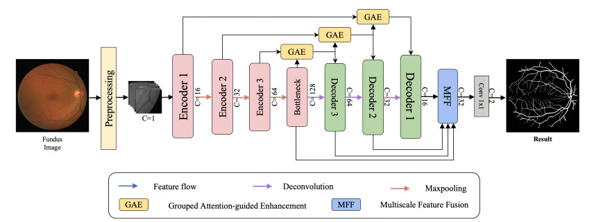
Retinal vessel segmentation plays a vital role in the clinical diagnosis of ophthalmic diseases. Despite convolutional neural networks (CNNs) excelling in this task, challenges persist, such as restricted receptive fields and information loss from downsampling. To address these issues, we propose a new multi-fusion network with grouped attention (MAG-Net). First, we introduce a hybrid convolutional fusion module instead of the original encoding block to learn more feature information by expanding the receptive field. Additionally, the grouped attention enhancement module uses high-level features to guide low-level features and facilitates detailed information transmission through skip connections. Finally, the multi-scale feature fusion module aggregates features at different scales, effectively reducing information loss during decoder upsampling. To evaluate the performance of the MAG-Net, we conducted experiments on three widely used retinal datasets: DRIVE, CHASE and STARE. The results demonstrate remarkable segmentation accuracy, specificity and Dice coefficients. Specifically, the MAG-Net achieved segmentation accuracy values of 0.9708, 0.9773 and 0.9743, specificity values of 0.9836, 0.9875 and 0.9906 and Dice coefficients of 0.8576, 0.8069 and 0.8228, respectively. The experimental results demonstrate that our method outperforms existing segmentation methods exhibiting superior performance and segmentation outcomes.

| [1] |
T. Xu, B. Wang, H. Liu, H. Wang, P. Yin, W. Dong, et al., Prevalence and causes of vision loss in China from 1990 to 2019: findings from the Global Burden of Disease Study 2019, Lancet Public Health, 5 (2020), e682–e691. https://doi.org/10.1016/S2468-2667(20)30254-1 doi: 10.1016/S2468-2667(20)30254-1

|
| [2] |
M. Mookiah, S. Hogg, T. J. MacGillivray, V. Prathiba, R. Pradeepa, V. Mohan, et al., A review of machine learning methods for retinal blood vessel segmentation and artery/vein classification, Med. Image Anal., 68 (2021), 101905. https://doi.org/10.1016/j.media.2020.101905 doi: 10.1016/j.media.2020.101905
|
| [3] |
C. Chen, J. H. Chuah, R. Ali, Y. Wang, Retinal vessel segmentation using deep learning: a review, IEEE Access, 9 (2021), 111985–112004. https://doi.org/10.1109/ACCESS.2021.310217 doi: 10.1109/ACCESS.2021.310217
|
| [4] |
C. L. Srinidhi, P. Aparna, J. Rajan, Recent advancements in retinal vessel segmentation, J. Med. Syst., 41 (2017), 1–22. https://doi.org/10.1007/s10916-017-0719-2 doi: 10.1007/s10916-017-0719-2
|
| [5] |
B. Zhang, L. Zhang, L. Zhang, F. Karray, Retinal vessel extraction by matched filter with first-order derivative of Gaussian, Comput. Biol. Med., 40 (2010), 438–445. https://doi.org/10.1016/j.compbiomed.2010.02.008 doi: 10.1016/j.compbiomed.2010.02.008
|
| [6] |
G. Hassan, N. El-Bendary, A. E. Hassanien, A. Fahmy, A. M. Shoeb, V. Snasel, Retinal blood vessel segmentation approach based on mathematical morphology, Procedia Comput. Sci., 65 (2015), 612–622. https://doi.org/10.1016/j.procs.2015.09.005 doi: 10.1016/j.procs.2015.09.005
|
| [7] |
F. Zana, J. C. Klein, Segmentation of vessel-like patterns using mathematical morphology and curvature evaluation, IEEE Trans. Image Process., 10 (2001), 1010–1019. https://doi.org/10.1109/83.931095 doi: 10.1109/83.931095
|
| [8] |
J. Zhao, J. Yang, D. Ai, H. Song, Y. Jiang, Y. Huang, et al., Automatic retinal vessel segmentation using multi-scale superpixel chain tracking, Digital Signal Process., 81 (2018), 26–42. https://doi.org/10.1016/j.dsp.2018.06.006 doi: 10.1016/j.dsp.2018.06.006
|
| [9] |
J. Yang, C. Lou, J. Fu, C. Feng, Vessel segmentation using multiscale vessel enhancement and a region based level set model, Comput. Med. Imaging Graphics, 85 (2020), 101783. https://doi.org/10.1016/j.compmedimag.2020.101783 doi: 10.1016/j.compmedimag.2020.101783
|
| [10] | J. Long, E. Shelhamer, T. Darrell, Fully convolutional networks for semantic segmentation, in Proceedings of the IEEE conference on computer vision and pattern recognition, (2015), 3431–3440. https://doi.org/10.1109/cvpr.2015.7298965 |
| [11] | H. Fu, Y. Xu, S. Lin, D. W. Wong, J. Liu, Deepvessel: Retinal vessel segmentation via deep learning and conditional random fiel, in Medical Image Computing and Computer-Assisted Intervention–MICCAI 2016: 19th International Conference, (2016), 132–139. https://doi.org/10.1007/978-3-319-46723-8_16 |
| [12] | O. Ronneberger, P. Fischer, T. Brox, U-net: Convolutional networks for biomedical image segmentation, in Medical Image Computing and Computer-Assisted Intervention–MICCAI 2015: 18th International Conference, (2015), 234–241. https://doi.org/10.1007/978-3-319-24574-4_28 |
| [13] | M. Entov, L. Polterovich, F. Zapolsky, Transunet: Transformers make strong encoders for medical image segmentation, preprint, arXiv: 2102.04306. |
| [14] | H. Cao, Y. Wang, J. Chen, D. Jiang, X. Zhang, Q. Tian, et al., Swin-unet: Unet-like pure transformer for medical image segmentation, in European Conference on Computer Vision, (2022), 205–218. https://doi.org/10.1007/978-3-031-25066-8_9 |
| [15] | S. Roy, G. Koehler, C. Ulrich, M. Baumgartner, J. Petersen, F. Isensee, et al., MedNeXt: Transformer-driven scaling of convNets for medical image segmentation, preprint, arXiv: 2303.09975. |
| [16] | A. Tragakis, C. Kaul, R. Murray-Smith, D. Husmeier, The fully convolutional transformer for medical image segmentation, in Proceedings of the IEEE/CVF Winter Conference on Applications of Computer Vision, (2023), 3660–3669. https://doi.org/10.1109/wacv56688.2023.00365 |
| [17] |
Y. Jiang, H. Zhang, N. Tan, L. Chen, Automatic retinal blood vessel segmentation based on fully convolutional neural networks, Symmetry, 11 (2019), 1112. https://doi.org/10.3390/sym11091112 doi: 10.3390/sym11091112
|
| [18] | A. Zhao, Image denoising with deep convolutional neural networks, Comput. Sci., 2016 (2016), 1–5. |
| [19] |
M. Z. Alom, C. Yakopcic, M. Hasan, T. M. Taha, V. K. Asari, Recurrent residual U-Net for medical image segmentation, J. Med. Imaging, 6 (2019), 014006. https://doi.org/10.1117/1.JMI.6.1.014006 doi: 10.1117/1.JMI.6.1.014006
|
| [20] | M. Zhang, F. Yu, J. Zhao, L. Zhang, Q. Li, BEFD: Boundary enhancement and feature denoising for vessel segmentation, in Medical Image Computing and Computer Assisted Intervention–MICCAI 2020: 23rd International Conference, (2020), 775–785. https://doi.org/10.1007/978-3-030-59722-1_75 |
| [21] | C. Guo, M. Szemenyei, Y. Yi, W. Wang, B. Chen, C. Fan, Sa-unet: Spatial attention u-net for retinal vessel segmentation, in 2020 25th international conference on pattern recognition (ICPR), (2021), 1236–1242. https://doi.org/10.1109/ICPR48806.2021.9413346 |
| [22] | W. Luo, Y. Li, R. Urtasun, R. Zemel, Understanding the effective receptive field in deep convolutional neural networks, Adv. Neural Inform. Process. Syst., 29 (2016). |
| [23] |
Q. Jin, Z. Meng, T. D. Pham, Q. Chen, L. Wei, DUNet: A deformable network for retinal vessel segmentation, Knowl. Based Syst., 178 (2019), 149–162. https://doi.org/10.1016/j.knosys.2019.04.025 doi: 10.1016/j.knosys.2019.04.025
|
| [24] |
H. Wu, W. Wang, J. Zhong, B. Lei, Z. Wen, J. Qin, Scs-net: A scale and context sensitive network for retinal vessel segmentation, Med. Image Anal., 70 (2021), 102025. https://doi.org/10.1016/j.media.2021.102025 doi: 10.1016/j.media.2021.102025
|
| [25] |
Z. Zhang, Y. Jiang, H. Qiao, M. Wang, W. Yan, SIL-Net: A Semi-Isotropic L-shaped network for dermoscopic image segmentation, Comput. Biol. Med., 150 (2022), 106146. https://doi.org/10.1016/j.compbiomed.2022.106146 doi: 10.1016/j.compbiomed.2022.106146
|
| [26] |
Y. Liu, J. Shen, L. Yang, G. Bian, H. Yu, ResDO-UNet: A deep residual network for accurate retinal vessel segmentation from fundus images, Biomed. Signal Process. Control, 79 (2023), 104087. https://doi.org/10.1016/j.bspc.2022.104087 doi: 10.1016/j.bspc.2022.104087
|
| [27] |
J. Cao, Y. Li, M. Sun, Y. Chen, D. Lischinski, D. Cohen-Or, et al., Do-conv: Depthwise over-parameterized convolutional layer, IEEE Trans. Image Process., 31 (2022), 3726–3736. https://doi.org/10.1109/TIP.2022.3175432 doi: 10.1109/TIP.2022.3175432
|
| [28] |
W. Zhou, W. Bai, J. Ji, Y. Yi, N. Zhang, W. Cui, Dual-path multi-scale context dense aggregation network for retinal vessel segmentation, Comput. Biol. Med., 164 (2023), 107269. https://doi.org/10.1016/j.compbiomed.2023.107269 doi: 10.1016/j.compbiomed.2023.107269
|
| [29] |
N. K. Tomar, D. Jha, M. A. Riegler, Fanet: A feedback attention network for improved biomedical image segmentation, IEEE Trans. Neural Networks Learn. Syst., 2022 (2022). https://doi.org/10.1109/TNNLS.2022.3159394 doi: 10.1109/TNNLS.2022.3159394
|
| [30] |
D. E. Alvarado-Carrillo, O. S. Dalmau-Cedeño, Width attention based convolutional neural network for retinal vessel segmentation, Expert Syst. Appl., 209 (2022), 118313. https://doi.org/10.1016/j.eswa.2022.118313 doi: 10.1016/j.eswa.2022.118313
|
| [31] |
M. Liu, Z. Wang, H. Li, P. Wu, F. E. Alsaadi, AA-WGAN: Attention augmented Wasserstein generative adversarial network with application to fundus retinal vessel segmentation, Comput. Biol. Med., 158 (2023), 106874. https://doi.org/10.1016/j.compbiomed.2023.106874 doi: 10.1016/j.compbiomed.2023.106874
|
| [32] |
M. R. Ahmed, M. Fahim, A. Islam, S. Islam, S. Shatabda, DOLG-NeXt: Convolutional neural network with deep orthogonal fusion of local and global features for biomedical image segmentation, Neurocomputing, 546 (2023), 126362. https://doi.org/10.1016/j.neucom.2023.126362 doi: 10.1016/j.neucom.2023.126362
|
| [33] |
J. Staal, M. D. Abràmoff, M. Niemeijer, M. A. Viergever, B. Van Ginneken, Ridge-based vessel segmentation in color images of the retina, IEEE Trans. Med. Imaging, 23 (20004), 501–509. https://doi.org/10.1109/TMI.2004.825627 doi: 10.1109/TMI.2004.825627
|
| [34] |
C. G. Owen, A. R. Rudnicka, R. Mullen, S. A. Barman, D. Monekosso, P. H. Whincup, et al., Measuring retinal vessel tortuosity in 10-year-old children: validation of the computer-assisted image analysis of the retina (CAIAR) program, Invest. Ophthalmol. Visual Sci., 50 (2009), 004–2010. https://doi.org/10.1167/iovs.08-3018 doi: 10.1167/iovs.08-3018
|
| [35] |
A. D. Hoover, V. Kouznetsova, M. Goldbaum, Locating blood vessels in retinal images by piecewise threshold probing of a matched filter response, IEEE Trans. Med. imaging, 19 (2000), 203–210. https://doi.org/10.1109/42.845178 doi: 10.1109/42.845178
|
| [36] | J. Hu, L. Shen, G. Sun, Squeeze-and-excitation networks, in Proceedings of the IEEE conference on computer vision and pattern recognition, (2018), 7132–7141. https://doi.org/10.1109/cvpr.2018.00745 |
| [37] | S. Woo, J. Park, J. Y. Lee, I. S. Kweon, Cbam: Convolutional block attention module, in Proceedings of the European conference on computer vision (ECCV), (2018), 3–19. https://doi.org/10.1007/978-3-030-01234-2_1 |
| [38] | Y. Cao, J. Xu, S. Lin, F. Wei, H. Hu, Gcnet: Non-local networks meet squeeze-excitation networks and beyond, in Proceedings of the IEEE/CVF international conference on computer vision workshops, 2019. https://doi.org/10.1109/iccvw.2019.00246 |
| [39] | O. Oktay, J. Schlemper, L. L. Folgoc, M. Lee, M. Heinrich, K. Misawa, et al., Attention u-net: Learning where to look for the pancreas, preprint, arXiv: 1804.03999. |
| [40] | M. Z. Alom, M. Hasan, C. Yakopcic, T. M. Taha, V. K. Asari, Recurrent residual convolutional neural network based on u-net (r2u-net) for medical image segmentation, preprint, arXiv: 1802.06955. |
| [41] |
Y. Wu, Y. Xia, Y. Song, Y. Zhang, W. Cai, NFN+: A novel network followed network for retinal vessel segmentation, Neural Networks, 126 (2020), 153–162. https://doi.org/10.1016/j.neunet.2020.02.018 doi: 10.1016/j.neunet.2020.02.018
|
| [42] |
Z. Lin, J. Huang, Y. Chen, X. Zhang, W. Zhao, Y. Li, A high resolution representation network with multi-path scale for retinal vessel segmentation, Comput. Methods Programs Biomed., 208 (2021), 106206. https://doi.org/10.1016/j.cmpb.2021.106206 doi: 10.1016/j.cmpb.2021.106206
|
| [43] |
Y. Yuan, L. Zhang, L. Wang, H. Huang, Multi-level attention network for retinal vessel segmentation, IEEE J. Biomed. Health Inform., 26 (2021), 312–323. https://doi.org/10.1109/JBHI.2021.3089201 doi: 10.1109/JBHI.2021.3089201
|
| [44] |
Y. Zhang, M. He, Z. Chen, K. Hu, X. Li, X. Gao, Bridge-Net: Context-involved U-net with patch-based loss weight mapping for retinal blood vessel segmentation, Expert Syst. Appl., 195 (2022), 116526. https://doi.org/10.1016/j.eswa.2022.116526 doi: 10.1016/j.eswa.2022.116526
|
| [45] |
F. Dong, D. Wu, C. Guo, S. Zhang, B. Yang, X. Gong, CRAUNet: A cascaded residual attention U-Net for retinal vessel segmentation, Comput. Biol. Med., 147 (2022), 105651. https://doi.org/10.1016/j.compbiomed.2022.105651 doi: 10.1016/j.compbiomed.2022.105651
|
| [46] |
B. Yang, L. Qin, H. Peng, C. Guo, X. Luo, J. Wang, SDDC-Net: A U-shaped deep spiking neural P convolutional network for retinal vessel segmentation, Digital Signal Process., 136 (2023), 104002. https://doi.org/10.1016/j.dsp.2023.104002 doi: 10.1016/j.dsp.2023.104002
|
| [47] |
Y. Jiang, W. Yan, J. Chen, H. Qiao, Z. Zhang, M. Wang, MS-CANet: Multi-Scale subtraction network with coordinate attention for retinal vessel segmentation, Symmetry, 15 (2023), 835. https://doi.org/10.3390/sym15040835 doi: 10.3390/sym15040835
|
| [48] |
J. Li, G. Gao, L. Yang, Y. Liu, GDF-Net: A multi-task symmetrical network for retinal vessel segmentation, Biomed. Signal Process. Control, 81 (2023), 104426. https://doi.org/10.1016/j.bspc.2022.104426 doi: 10.1016/j.bspc.2022.104426
|
| [49] |
T. M. Khan, S. S. Naqvi, A. Robles-Kelly, I. Razzak, Retinal vessel segmentation via a Multi-resolution Contextual Network and adversarial learning, Neural Networks, 2023 (2023). https://doi.org/10.1016/j.neunet.2023.05.029 doi: 10.1016/j.neunet.2023.05.029
|


Figures(9) / Tables(9)

Yun Jiang, Jie Chen, Wei Yan, Zequn Zhang, Hao Qiao, Meiqi Wang. MAG-Net : Multi-fusion network with grouped attention for retinal vessel segmentation[J]. Mathematical Biosciences and Engineering, 2024, 21(2): 1938-1958. doi: 10.3934/mbe.2024086


 DownLoad: