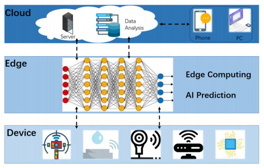
Unusual states of manhole covers (MCs), such as being tilted, lost or flooded, can present substantial safety hazards and risks to pedestrians and vehicles on the roadway. Most MCs are still being managed through manual regular inspections and have limited information technology integration. This leads to time-consuming and labor-intensive identification with a lower level of accuracy. In this paper, we propose an edge computing-based intelligent monitoring system for manhole covers (EC-MCIMS). Sensors detect the MC and send status and positioning information via LoRa to the edge gateway located on the nearby wisdom pole. The edge gateway utilizes a lightweight machine learning model, trained on the edge impulse (EI) platform, which can predict the state of the MC. If an abnormality is detected, the display and voice device on the wisdom pole will respectively show and broadcast messages to alert pedestrians and vehicles. Simultaneously, the information is uploaded to the cloud platform, enabling remote maintenance personnel to promptly repair and restore it. Tests were performed on the EI platform and in Dongguan townships, demonstrating that the average response time for identifying MCs is 4.81 s. Higher responsiveness and lower power consumption were obtained compared to cloud computing models. Moreover, the system utilizes a lightweight model that better reduces read-only memory (ROM) and random-access memory (RAM), while maintaining an average identification accuracy of 94%.
Citation: Liang Yu, Zhengkuan Zhang, Yangbing Lai, Yang Zhao, Fu Mo. Edge computing-based intelligent monitoring system for manhole cover[J]. Mathematical Biosciences and Engineering, 2023, 20(10): 18792-18819. doi: 10.3934/mbe.2023833
Unusual states of manhole covers (MCs), such as being tilted, lost or flooded, can present substantial safety hazards and risks to pedestrians and vehicles on the roadway. Most MCs are still being managed through manual regular inspections and have limited information technology integration. This leads to time-consuming and labor-intensive identification with a lower level of accuracy. In this paper, we propose an edge computing-based intelligent monitoring system for manhole covers (EC-MCIMS). Sensors detect the MC and send status and positioning information via LoRa to the edge gateway located on the nearby wisdom pole. The edge gateway utilizes a lightweight machine learning model, trained on the edge impulse (EI) platform, which can predict the state of the MC. If an abnormality is detected, the display and voice device on the wisdom pole will respectively show and broadcast messages to alert pedestrians and vehicles. Simultaneously, the information is uploaded to the cloud platform, enabling remote maintenance personnel to promptly repair and restore it. Tests were performed on the EI platform and in Dongguan townships, demonstrating that the average response time for identifying MCs is 4.81 s. Higher responsiveness and lower power consumption were obtained compared to cloud computing models. Moreover, the system utilizes a lightweight model that better reduces read-only memory (ROM) and random-access memory (RAM), while maintaining an average identification accuracy of 94%.

| [1] |
W. Liu, D. Y. Chen, P. C. Yin, M. Y. Yang, E. Z. Li, M. Xie, et al., Small manhole cover detection in remote sensing imagery with deep convolutional neural networks, ISPRS. Int. J. Geo-Inf., 8 (2019), 913–924. https://doi.org/10.3390/ijgi8010049 doi: 10.3390/ijgi8010049

|
| [2] |
B. D. Zhou, W. J. Zhao, W. H. Guo, L. C. Li, D. J. Zhang, Q. Z. Mao, et al., Smartphone-based road manhole cover detection and classification, Autom. Constr., 140 (2022), 104344–104355. https://doi.org/10.1016/j.autcon.2022.104344 doi: 10.1016/j.autcon.2022.104344
|
| [3] |
R. Hubaut, R. Guichard, J. Greenfield, M. Blandeau, Validation of an embedded motion-capture and EMG setup for the analysis of musculoskeletal disorder risks during manhole cover handling, Sensors, 22 (2022), 436–451. https://doi.org/10.3390/s22020436 doi: 10.3390/s22020436
|
| [4] |
V. Albino, U. Berardi, R. M. Dangelico, Smart cities: Definitions, dimensions, performance, and initiatives, J. Urban Technol., 22 (2015), 3–21. https://doi.org/10.1080/10630732.2014.942092 doi: 10.1080/10630732.2014.942092
|
| [5] |
X. Y. Liu, Y. Han, Y. H. Du, IoT device identification using directional packet length sequences and 1D-CNN, Sensors, 22 (2022), 8337–8356. https://doi.org/10.3390/s22218337 doi: 10.3390/s22218337
|
| [6] | S. Hymel, C. Banbury, D. Situnayake, A. Elium, C. Ward, M. Kelcey, et al., Edge Impulse: An MLOps platform for tiny machine learning, preprint, arXiv: 2212.03332. |
| [7] | H. H. Aly, A. H. Soliman, M. Mouniri, Towards a fully automated monitoring system for manhole cover: Smart cities and IOT applications, in 2015 IEEE First International Smart Cities Conference (ISC2), (2015), 1–7. https://doi.org/10.1109/ISC2.2015.7366150 |
| [8] | X. R. Fu, Manhole cover intelligent detection and management system, in 2016 6th International Conference on Electronic, Mechanical, Information and Management Society (ICEMIMS), (2016), 986–988. https://doi.org/10.2991/emim-16.2016.203 |
| [9] | V. K. Nallamothu, S. Medidi, S. P. Jannu, IOT based manhole detection and monitoring system, in 2022 International Conference on Distributed Computing and Electrical Circuits and Electronics (ICDCECE), (2022), 1–6. https://doi.org/10.1109/ICDCECE53908.2022.9793287 |
| [10] | R. Dronavalli, K. Seelam, P. Maganti, J. Gowineni, S. D. Challamalla, IoT-based automatic manhole observant for sewage worker's safety, in 2022 International Conference on Automation, Computing and Renewable Systems (ICACRS), (2022), 310–316. https://doi.org/10.1109/ICACRS55517.2022.10029252 |
| [11] | S. Salehin, S. S. Akter, A. Ibnat, T. T. Anannya, N. N. Liya, M. Paramita, et al., An IoT based proposed system for monitoring manhole in context of Bangladesh, in 2018 4th International Conference on Electrical Engineering and Information & Communication Technology (ICEEICT), (2018), 411–415. https://doi.org/10.1109/CEEICT.2018.8628091 |
| [12] |
C. S. Ram, C. N. Kumar, S. Abhilash, Automated street light control and manhole monitoring with fault detection & reporting system for municipal department, Int. J. Sci. Res. Eng. Man, 7 (2023), 9–15. https://doi.org/10.55041/IJSREM.17962 doi: 10.55041/IJSREM.17962
|
| [13] |
S. K. Muragesh, R. Santhosha, Automated internet of things for underground drainage and manhole monitoring system for metropolitan cities, Int. J. Inf. Comput. Technol., 4 (2014), 1211–1220. https://doi.org/10.0974/IJICT.15634 doi: 10.0974/IJICT.15634
|
| [14] | Y. Liu, M. Y. Du, C. F. Jing, Y. Bai, Design of supervision and management system for ownerless manhole covers based on RFID, in 2013 21st International Conference on Geoinformatics (ICG), (2013), 1–4. https://doi.org/10.1109/Geoinformatics.2013.6626149 |
| [15] |
G. Y. Jia, G. J. Han, H. L. Rao, L. Shu, Edge computing-based intelligent manhole cover management system for smart cities, IEEE Internet Things, 5 (2018), 1648–1656. https://doi.org/10.1109/JIOT.2017.2786349 doi: 10.1109/JIOT.2017.2786349
|
| [16] |
A. Mankotia, A. K. Shukla, IOT based manhole detection and monitoring system using Arduino, Mater. Today: Proc., 57 (2022), 2195–2198. https://doi.org/10.1016/j.matpr.2021.12.264 doi: 10.1016/j.matpr.2021.12.264
|
| [17] | N. Nataraja, R. Amruthavarshini, N. L. Chaitra, K. Jyothi, N. Krupaa, S. S. M. Saqquaf, Secure manhole monitoring system employing sensors and GSM techniques, in 2018 3rd IEEE International Conference on Recent Trends in Electronics, Information & Communication Technology (RTEICT), (2018), 2078–2082. https://doi.org/10.1109/RTEICT42901.2018.9012245 |
| [18] | X. C. Guo, B. B. Liu, L. L. Wang, Design and implementation of intelligent manhole cover monitoring system based on NB-IoT, in 2019 International Conference on Robots & Intelligent System (ICRIS), (2019), 207–210. https://doi.org/10.1109/ICRIS.2019.00061 |
| [19] | J. P. Zhang, X. L. Zeng, Design of intelligent manhole cover monitoring system based on narrow band internet of things, in 2022 7th International Conference on Intelligent Computing and Signal Processing (ICSP), (2022), 1354–1357. https://doi.org/10.1109/ICSP54964.2022.9778462 |
| [20] |
W. Sun, Design and realization of LoRa-based manhole cover safety monitoring system, J. Int. Things Technol., 9 (2019), 25–26, 30. https://doi.org/10.16667/j.issn.2095-1302.2019.04.005 doi: 10.16667/j.issn.2095-1302.2019.04.005
|
| [21] |
H. S. Zhang, L. Li, X. Liu, Development and test of manhole cover monitoring device using LoRa and accelerometer, IEEE Trans. Instrum. Meas., 69 (2020), 2570–2580. https://doi.org/10.1109/TIM.2020.2967854 doi: 10.1109/TIM.2020.2967854
|
| [22] | X. Liu, H. S. Zhang, L. Li, Research on LoRa communication performance in manhole cover monitoring, in 2019 IEEE International Instrumentation and Measurement Technology Conference (I2MTC), (2019), 1–6. https://doi.org/10.1109/I2MTC.2019.8826898 |
| [23] | L. Li, H. S. Zhang, X. Liu, Development of low power consumption manhole cover monitoring device using LoRa, in 2019 IEEE International Instrumentation and Measurement Technology Conference (I2MTC), (2019), 1–6. https://doi.org/10.1109/I2MTC.2019.8826885 |
| [24] | Y. Yu, J. Li, H. Guan, C. Wang, Automated detection of road manhole covers from mobile LiDAR point-clouds based on a marked point process, in 2013 Fifth International Conference on Geo-Information Technologies for Natural Disaster Management (ICGITNDM), (2013), 130–136. https://doi.org/10.1109/GIT4NDM.2013.23 |
| [25] |
Z. Y. Wei, M. M. Yang, L. Z. Wang, H. Ma, X. X. Chen, R. F. Zhong, Customized mobile LiDAR system for manhole cover detection and identification, Sensors, 19 (2019), 2422–2439. https://doi.org/10.3390/s19102422 doi: 10.3390/s19102422
|
| [26] | V. Vishnani, A. Adhya, C. Bajpai, P. Chimurkar, K. Khandagle, Manhole detection using image processing on google street view imagery, in 2020 Third International Conference on Smart Systems and Inventive Technology (ICSSIT), (2020), 684–688. https://doi.org/10.1109/ICSSIT48917.2020.9214219 |
| [27] | U. Andrijašević, J. Kocić, V. Nešić, Lid opening detection in manholes using RNN, in 2020 28th Telecommunications Forum (TELFOR), (2020), 1–4. https://doi.org/10.1109/TELFOR51502.2020.9306668 |
| [28] |
R. Krishnan, A. Santhana, D. D. Kumari, N. Nandhini, G. Karpagarajesh, K. Narayanan, et al., A secured manhole management system using IoT and machine learning, Rec. Adv. Int. Things Mach. Learn., 215 (2022), 3–22. https://doi.org/10.1007/978-3-030-90119-6_3 doi: 10.1007/978-3-030-90119-6_3
|
| [29] |
D. P. Zhang, X. C. Yu, L. Yang, D. Y. Quan, H. M. Mi, K. Yan, Data-augmented deep learning models for abnormal road manhole cover detection, Sensors, 23 (2023), 2676–2693. https://doi.org/10.3390/s23052676 doi: 10.3390/s23052676
|
| [30] | K. Thakur, A. Adhya, C. Bajpai, P. Chimurkar, P. Kasambe, Manhole management using image processing and data analytics, in 2021 12th International Conference on Computing Communication and Networking Technologies (ICCCNT), 12 (2021), 1–5. https://doi.org/10.1109/ICCCNT51525.2021.9579541 |
| [31] |
W. S. Shi, J. Cao, Q. Zhang, Y. H. Z. Li, L. Y. Xu, Edge computing: Vision and challenges, IEEE Internet Things, 3 (2016), 637–646. https://doi.org/10.1109/JIOT.2016.2579198 doi: 10.1109/JIOT.2016.2579198
|
| [32] |
F. Mo, L. Yu, Z. K. Zhang, Y. Zhao, Design and implementation of manhole cover safety monitoring system based on smart light pole, Math. Probl. Eng., 2022 (2022), 1–12. https://doi.org/10.1155/2022/3081649 doi: 10.1155/2022/3081649
|
| [33] |
B. Ravelo, M. Guerin, W. Rahajandraibe, V. Gies, L. Rajaoarisoa, S. Lalléchère, Low-pass NGD numerical function and STM32 MCU emulation test, IEEE Trans. Ind. Electron., 8 (2022), 8346–8355. https://doi.org/10.1109/TIE.2021.3109543 doi: 10.1109/TIE.2021.3109543
|
| [34] |
V. B. Vales, O. C. Fernández, T. D. Bolaño, C. J. Escudero, J. A. G. Naya, Fine time measurement for the internet of things: a practical approach using ESP32, IEEE Internet Things, 19 (2022), 18305–18318. https://doi.org/10.1109/JIOT.2022.3158701 doi: 10.1109/JIOT.2022.3158701
|
| [35] |
W. S. Shi, X. Z. Zhang, Y. F. Wang, Q. Y. Zhang, Edge computing: Status and prospects, J. Comput. Res. Dev., 56 (2019), 69–89. https://doi.org/10.7544/issn1000-1239.2019.20180760 doi: 10.7544/issn1000-1239.2019.20180760
|
| [36] |
W. S. Shi, H. Sun, J. Cao, Q. Zhang, W. Liu, Edge computing: A new computing model for the internet of everything era, J. Comput. Res. Dev., 54 (2017), 907–924. https://doi.org/10.7544/issn1000-1239.2017.20160941 doi: 10.7544/issn1000-1239.2017.20160941
|
| [37] |
Y. F. Li, X. R. He, Y. Z. Bian, Task offloading of edge computing network and energy saving of passive house for smart city, Mob. Inf. Syst., 2022 (2022), 1–11. https://doi.org/10.1155/2022/4832240 doi: 10.1155/2022/4832240
|
| [38] |
B. Pang, E. Nijkamp, Y. N. Wu, Deep learning with TensorFlow: A review, J. Educ. Behav. Stat., 2 (2020), 227–248. https://doi.org/10.3102/1076998619872761 doi: 10.3102/1076998619872761
|
| [39] |
I. N. Mihigo, M. Zennaro, A. Uwitonze, J. Rwigema, M. Rovai, On-Device IoT-based predictive maintenance analytics model: Comparing TinyLSTM and TinyModel from edge impulse, Sensors, 22 (2022), 5174–5194. https://doi.org/10.3390/s22145174 doi: 10.3390/s22145174
|
| [40] | L. Qing, K. Yang, W. Tan, J. Li, Automated detection of manhole covers in Mls point clouds using a deep learning approach, in IGARSS 2020-2020 IEEE International Geoscience and Remote Sensing Symposium, (2020), 1580–1583. https://doi.org/10.1109/IGARSS39084.2020.9324137 |
| [41] |
S. J. Tian, S. Wang, H. R. Xu, Early detection of freezing damage in oranges by online Vis/NIR computers and electronics in agriculture transmission coupled with diameter correction method and deep 1D-CNN, Comput. Electr. Agric., 193 (2022), 106638–106659. https://doi.org/10.1016/j.compag.2021.106638 doi: 10.1016/j.compag.2021.106638
|
| [42] |
C. C. Che, H. W. Wang, X. M. Ni, R. G. Ning, M. L. Xiong, Remaining life prediction of aero-engine based on 1D-CNN and Bi-LSTM, J. Mech. Eng., 57 (2021), 304–312. https://doi.org/10.3901/JME.2021.14.304 doi: 10.3901/JME.2021.14.304
|
| [43] | Y. Kim, Convolutional neural networks for sentence classification, preprint, arXiv: 1408.5882. |
| [44] |
H. J. Wang, Z. Y. Yi, Z. Z. Ke, Y. J. Guo, H. Y. Dong, Wear monitoring of spiral milling tools based on one-dimensional convolutional neural network, J. Zhejiang Univ. (Eng. Ed.), 54 (2020), 931–939. https://doi.org/10.3785/j.issn.1008-973X.2020.05.010 doi: 10.3785/j.issn.1008-973X.2020.05.010
|
| [45] |
L. Liu, J. C. Zhu, G. J. Han, Y. G. Bi, Bearing health monitoring and fault diagnosis based on joint feature extraction in one-dimensional convolution neural network, J. Soft., 32 (2021), 2379−2390. https://doi.org/10.13328/j.cnki.jos.006188 doi: 10.13328/j.cnki.jos.006188
|
| [46] |
H. T. Ren, F. Deng, Manhole cover detection using depth information, J. Phys.: Conf. Ser., 1856 (2021), 1–7. https://doi.org/10.1088/1742-6596/1856/1/012037 doi: 10.1088/1742-6596/1856/1/012037
|
| [47] |
W. M. Rasheed, R. Abdulla, L. Y. San, Manhole cover monitoring system over IOT, J. Appl. Technol. Innov., 5 (2021), 1–6. https://doi.org/10.2600/JATI.245739682 doi: 10.2600/JATI.245739682
|
| [48] | S. Bouhoula, M. Avgeris, A. Leivadeas, I. Lambadaris, Computational offloading for the industrial internet of things: A performance analysis, in 2022 IEEE International Mediterranean Conference on Communications and Networking (MeditCom), (2022), 1–6. https://doi.org/10.1109/MeditCom55741.2022.9928770 |


Figures(25) / Tables(3)

Liang Yu, Zhengkuan Zhang, Yangbing Lai, Yang Zhao, Fu Mo. Edge computing-based intelligent monitoring system for manhole cover[J]. Mathematical Biosciences and Engineering, 2023, 20(10): 18792-18819. doi: 10.3934/mbe.2023833


 DownLoad: