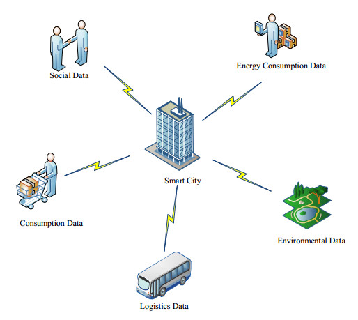
The fire safety management policy is the premise for city managers to master the urban fire safety situation and solve the urban fire safety problems. An excellent fire safety management policy can obtain the basic data of fire safety, analyze the existing problems and potential safety hazards, and provide targeted measures for urban fire safety management. At present, the traditional fire safety management policy has exposed many shortcomings, such as the lack of technical support for firefighting means, inaccurate fire data analysis, etc., which ultimately led to low fire extinguishing efficiency and wasted some human and material resources. In the context of smart cities, big data (BD) and artificial intelligence (AI) have gradually integrated into various fields of urban development. This paper studied the fire safety management policies of smart cities based on BD analysis method. First, it summarized the relationship among BD, AI and smart cities, then analyzed the limitations of traditional urban fire safety management models, and finally proposed new fire safety management methods based on BD, AI and sustainable development. This article analyzed the urban fire protection situation from January to June 2022 in Nanchang, and verified the effectiveness of the method proposed in this article. Research has shown that the new fire safety management policy has reduced the number of fires, improved fire extinguishing efficiency by 9.07%, reduced property damage and casualties, and has a high recognition of the method. This also provides a reference for the next step of BD's application in smart cities.
Citation: Xiaodong Qian. Evaluation on sustainable development of fire safety management policies in smart cities based on big data[J]. Mathematical Biosciences and Engineering, 2023, 20(9): 17003-17017. doi: 10.3934/mbe.2023758
The fire safety management policy is the premise for city managers to master the urban fire safety situation and solve the urban fire safety problems. An excellent fire safety management policy can obtain the basic data of fire safety, analyze the existing problems and potential safety hazards, and provide targeted measures for urban fire safety management. At present, the traditional fire safety management policy has exposed many shortcomings, such as the lack of technical support for firefighting means, inaccurate fire data analysis, etc., which ultimately led to low fire extinguishing efficiency and wasted some human and material resources. In the context of smart cities, big data (BD) and artificial intelligence (AI) have gradually integrated into various fields of urban development. This paper studied the fire safety management policies of smart cities based on BD analysis method. First, it summarized the relationship among BD, AI and smart cities, then analyzed the limitations of traditional urban fire safety management models, and finally proposed new fire safety management methods based on BD, AI and sustainable development. This article analyzed the urban fire protection situation from January to June 2022 in Nanchang, and verified the effectiveness of the method proposed in this article. Research has shown that the new fire safety management policy has reduced the number of fires, improved fire extinguishing efficiency by 9.07%, reduced property damage and casualties, and has a high recognition of the method. This also provides a reference for the next step of BD's application in smart cities.

| [1] |
N. M. Salleh, N. A. A. Salim, M. Jaafar, M. Z. Sulieman, A. Ebekozien, Fire safety management of public buildings: A systematic review of hospital buildings in Asia, Prop. Manage., 38 (2020), 497–511. https://doi.org/10.1108/PM-12-2019-0069 doi: 10.1108/PM-12-2019-0069

|
| [2] |
G. Spinardi, J. Baker, L. Bisby, Post construction fire safety regulation in England: shutting the door before the horse has bolted, Policy Pract. Health Safety, 17 (2019), 133–145. https://doi.org/10.1080/14773996.2019.1591040 doi: 10.1080/14773996.2019.1591040
|
| [3] |
M. K. Alao, Y. M. Yatim, W. Y. W. Mahmood, Fire safety management strategy in Nigeria public buildings, Jurnal Kejuruteraan, 33 (2021), 663–671. https://doi.org/10.17576/jkukm-2021-33(3)-24 doi: 10.17576/jkukm-2021-33(3)-24
|
| [4] |
C. M. Benson, S. Elsmore, Reducing fire risk in buildings: the role of fire safety expertise and governance in building and planning approval, J. Hous. Built Environ., 37 (2022), 927–950. https://doi.org/10.1007/s10901-021-09870-9 doi: 10.1007/s10901-021-09870-9
|
| [5] | I. Y. Ebenehi, S. Mohamed, N. Sarpin, S. T. Wee, A. A. Adaji, Building users' appraisal of effective fire safety management for building facilities in Malaysian higher education institutions: A pilot study, Traektoria Nauki = Path Sci., 4 (2018), 2001–2010. |
| [6] |
R. Roslan, S. Y. Said, Fire safety management system for heritage buildings in Malaysia. Environ.-Behav. Proc. J., 2 (2017), 221–226. https://doi.org/10.21834/e-bpj.v2i6.961 doi: 10.21834/e-bpj.v2i6.961
|
| [7] | P. Mutinda, P. Karanja, P. Makhonge, Assessment of fire safety management and adequacy of the existing control measures in Kenya power; Nairobi region, J. Agr. Sci. Tech., 18 (2017), 63–96. |
| [8] |
P. Agarwal, J. Tang, A. N. L. Narayanan, J. Zhuang, Big data and predictive analytics in fire risk using weather data, Risk Anal., 40 (2020), 1438–1449. https://doi.org/10.1111/risa.13480 doi: 10.1111/risa.13480
|
| [9] |
J. S. Kim, B. S. Kim, Analysis of fire-accident factors using big-data analysis method for construction areas, KSCE J. Civ. Eng., 22 (2018), 1535–1543. https://doi.org/10.1007/s12205-017-0767-7 doi: 10.1007/s12205-017-0767-7
|
| [10] |
Y. Lu, Z. Zhao, X. Jiang, J. Wu, X. Fan, Dynamic fire risk indexes for stadiums from perspective of big data, China Safety Sci. J., 32 (2022), 155–162. https://doi.org/10.16265/j.cnki.issn1003-3033.2022.04.023 doi: 10.16265/j.cnki.issn1003-3033.2022.04.023
|
| [11] |
W. Khalid, M. Burneo, L. Hvam, A framework for multiple fire investigation using big data and statistical analysis, J. Fail. Anal. Prev., 21 (2021), 890–903. https://doi.org/10.1007/s11668-021-01125-7 doi: 10.1007/s11668-021-01125-7
|
| [12] |
E. Park, S. Min, Standardization of fire factor for big data, J. Korean Soc. Hazard Mitig., 19 (2019), 143–149. https://doi.org/10.9798/KOSHAM.2019.19.4.143 doi: 10.9798/KOSHAM.2019.19.4.143
|
| [13] | H. J. Joo, Y. J. Choi, C. Y. Ok, J. H. An, Determination of fire risk assessment indicators for building using big data, J. Korea Inst. Build. Constr., 22 (2022), 281–291. |
| [14] | F. Zhang, J. Huang, Intelligent early warning system for ecological forest fire based on big data, Ekoloji, 28 (2019), 2033–2037. |
| [15] |
X. Li, H. Liu, W. Wang, Y. Zheng, H. Lv, Z. Lv, Big data analysis of the internet of things in the digital twins of smart city based on deep learning, Future Gener. Comput. Syst., 128 (2021), 167–177. https://doi.org/10.1016/j.future.2021.10.006 doi: 10.1016/j.future.2021.10.006
|
| [16] | A. I. Voda, L. D. Radu, Artificial intelligence and the future of smart cities, BRAIN-Broad Res. Arti., 9 (2018), 110–127. |
| [17] |
M. Z. Naser, Mechanistically informed machine learning and artificial intelligence in fire engineering and sciences, Fire Technol., 57 (2021), 2741–2784. https://doi.org/10.1007/s10694-020-01069-8 doi: 10.1007/s10694-020-01069-8
|
| [18] |
V. Kodur, P. Kumar, M. M. Rafi, Fire hazard in buildings: review, assessment and strategies for improving fire safety, PSU Res. Rev., 4 (2020), 1–23. https://doi.org/10.1108/PRR-12-2018-0033 doi: 10.1108/PRR-12-2018-0033
|
| [19] |
P. Agarwal, J. Tang, A. N. L. Narayanan, J. Zhuang, Big data and predictive analytics in fire risk using weather data, Risk Anal., 40 (2020), 1438–1449. https://doi.org/10.1111/risa.13480 doi: 10.1111/risa.13480
|
| [20] |
W. Jin, Y. Liu, Y. Jin, M. Jia, L. Xue, The construction of builder safety supervision system based on CPS, Wirel. Commun. Mob. Comput., 2020 (2020), 1–11. https://doi.org/10.1155/2020/8856831 doi: 10.1155/2020/8856831
|
| [21] |
G. Sun, S. Wang, H. Wang, Y. Gao, Research on the construction of intelligent fire protection virtual simulation teaching platform based on internet of things, Int. J. Inform. Educ. Technol., 11 (2021), 450–455. https://doi.org/10.18178/ijiet.2021.11.10.1549 doi: 10.18178/ijiet.2021.11.10.1549
|
| [22] | A. C. Chavez, High performance computing for big data in distributed systems, Distrib. Proc. Syst., 1 (2020), 10–17. |
| [23] | S. Y. Ding, H. Yang, Discussion on the technology of fire risk forecast driven by big data, Fire Sci. Technol., 39 (2020), 1743. |
| [24] |
S. Saponara, A. Elhanashi, A. Gagliardi, Real-time video fire/smoke detection based on CNN in antifire surveillance systems, J. Real-Time Image Proc., 18 (2021), 889–900. https://doi.org/10.1007/s11554-020-01044-0 doi: 10.1007/s11554-020-01044-0
|
| [25] |
X. Wu, Y. Park, A. Li, X. Huang, F. Xiao, A Usmani Smart detection of fire source in tunnel based on the numerical database and artificial intelligence, Fire Technol., 57 (2021), 657–682. https://doi.org/10.1007/s10694-020-00985-z doi: 10.1007/s10694-020-00985-z
|
| [26] | W. B. Horng, J. W. Peng, C. Y. Chen, A new image-based real-time flame detection method using color analysis, in Proceedings. 2005 IEEE Networking, Sensing and Control, (2005), 100–105. https://doi.org/10.1109/ICNSC.2005.1461169 |


Figures(6) / Tables(1)

Xiaodong Qian. Evaluation on sustainable development of fire safety management policies in smart cities based on big data[J]. Mathematical Biosciences and Engineering, 2023, 20(9): 17003-17017. doi: 10.3934/mbe.2023758


 DownLoad: