Robust capped norm dual hyper-graph regularized non-negative matrix tri-factorization

Jiyang Yu; Baicheng Pan; Shanshan Yu; Man-Fai Leung; Jiyang Yu; Baicheng Pan; Shanshan Yu; Man-Fai Leung

doi:10.3934/mbe.2023556

Mathematical Biosciences and Engineering

2023, Volume 20, Issue 7: 12486-12509. doi: 10.3934/mbe.2023556

Previous Article Next Article

Research article Special Issues

Robust capped norm dual hyper-graph regularized non-negative matrix tri-factorization

1.
College of Electronic and Information Engineering, Southwest University, Chongqing 400715, China
2.
Chongqing Key Laboratory of Nonlinear Circuits and Intelligent Information Processing, College of Electronic and Information Engineering, Southwest University, Chongqing 400715, China
3.
Training and Basic Education Management Office, Southwest University, Chongqing 400715, China
4.
School of Computing and Information Science, Faculty of Science and Engineering, Anglia Ruskin University, Cambridge, United Kingdom

Academic Editor: Keping Yu

Received: 13 February 2023 Revised: 24 April 2023 Accepted: 15 May 2023 Published: 24 May 2023

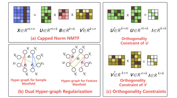
Non-negative matrix factorization (NMF) has been widely used in machine learning and data mining fields. As an extension of NMF, non-negative matrix tri-factorization (NMTF) provides more degrees of freedom than NMF. However, standard NMTF algorithm utilizes Frobenius norm to calculate residual error, which can be dramatically affected by noise and outliers. Moreover, the hidden geometric information in feature manifold and sample manifold is rarely learned. Hence, a novel robust capped norm dual hyper-graph regularized non-negative matrix tri-factorization (RCHNMTF) is proposed. First, a robust capped norm is adopted to handle extreme outliers. Second, dual hyper-graph regularization is considered to exploit intrinsic geometric information in feature manifold and sample manifold. Third, orthogonality constraints are added to learn unique data presentation and improve clustering performance. The experiments on seven datasets testify the robustness and superiority of RCHNMTF.
- non-negative matrix tri-factorization,
- capped norm,
- dual hyper-graph regularization,
- robust clustering
Citation: Jiyang Yu, Baicheng Pan, Shanshan Yu, Man-Fai Leung. Robust capped norm dual hyper-graph regularized non-negative matrix tri-factorization[J]. Mathematical Biosciences and Engineering, 2023, 20(7): 12486-12509. doi: 10.3934/mbe.2023556

Related Papers:

Abstract

Non-negative matrix factorization (NMF) has been widely used in machine learning and data mining fields. As an extension of NMF, non-negative matrix tri-factorization (NMTF) provides more degrees of freedom than NMF. However, standard NMTF algorithm utilizes Frobenius norm to calculate residual error, which can be dramatically affected by noise and outliers. Moreover, the hidden geometric information in feature manifold and sample manifold is rarely learned. Hence, a novel robust capped norm dual hyper-graph regularized non-negative matrix tri-factorization (RCHNMTF) is proposed. First, a robust capped norm is adopted to handle extreme outliers. Second, dual hyper-graph regularization is considered to exploit intrinsic geometric information in feature manifold and sample manifold. Third, orthogonality constraints are added to learn unique data presentation and improve clustering performance. The experiments on seven datasets testify the robustness and superiority of RCHNMTF.

References

[1]	I. T. Jolliffe, J. Cadima, in Principal component analysis: a review and recent developments, Philosophical transactions of the Royal Society A: Mathematical, Physical and Engineering Sciences, 374 (2016), 20150202. https://doi.org/10.1098/rsta.2015.0202
[2]	R. O. Duda, P. E. Hart, Pattern Classification, John Wiley & Sons, 2006.
[3]	A. Gersho, R. M. Gray, Vector Quantization and Signal Compression, Springer Science & Business Media, 2012.
[4]	D. Seung, L. Lee, Algorithms for non-negative matrix factorization, Adv. Neural Inf. Process. Syst., 13 (2001), 556–562.
[5]	D. Li, S. Zhang, X. Ma, Dynamic module detection in temporal attributed networks of cancers, IEEE/ACM Trans. Comput. Biol. Bioinf., 19 (2021), 2219–2230. https://doi.org/10.1109/TCBB.2021.3069441 doi: 10.1109/TCBB.2021.3069441
[6]	Z. Zhao, Z. Ke, Z. Gou, H. Guo, K. Jiang, R. Zhang, The trade-off between topology and content in community detection: An adaptive encoder–decoder-based nmf approach, Expert Syst. Appl., 209 (2022), 118230. https://doi.org/10.1016/j.eswa.2022.118230 doi: 10.1016/j.eswa.2022.118230
[7]	N. Yu, M. J. Wu, J. X. Liu, C. H. Zheng, Y. Xu, Correntropy-based hypergraph regularized nmf for clustering and feature selection on multi-cancer integrated data, IEEE Trans. Cybern., 51 (2020), 3952–3963. https://doi.org/10.1109/TCYB.2020.3000799 doi: 10.1109/TCYB.2020.3000799
[8]	N. Yu, Y. L. Gao, J. X. Liu, J. Wang, J. Shang, Hypergraph regularized nmf by l 2, 1-norm for clustering and com-abnormal expression genes selection, in 2018 IEEE International Conference on Bioinformatics and Biomedicine (BIBM), (2018), 578–582.
[9]	M. Venkatasubramanian, K. Chetal, D. J. Schnell, G. Atluri, N. Salomonis, Resolving single-cell heterogeneity from hundreds of thousands of cells through sequential hybrid clustering and nmf, Bioinformatics, 36 (2020), 3773–3780. https://doi.org/10.1093/bioinformatics/btaa201 doi: 10.1093/bioinformatics/btaa201
[10]	W. Wu, X. Ma, Network-based structural learning nonnegative matrix factorization algorithm for clustering of scrna-seq data, IEEE/ACM Trans. Comput. Biol. Bioinf., 20 (2022), 566–575. https://doi.org/10.1038/s41579-022-00790-1 doi: 10.1038/s41579-022-00790-1
[11]	R. Egger, J. Yu, A topic modeling comparison between lda, nmf, top2vec, and bertopic to demystify twitter posts, Front. Soc., 7 (2022).
[12]	H. Che, J. Wang, Nonnegative matrix factorization algorithm based on a discrete-time projection neural network, Neural Networks, 103 (2018), 63–71. https://doi.org/10.1016/j.neunet.2018.03.003 doi: 10.1016/j.neunet.2018.03.003
[13]	H. Che, J. Wang, A. Cichocki, Bicriteria sparse nonnegative matrix factorization via two-timescale duplex neurodynamic optimization, IEEE Trans. Neural Networks Learn. Syst., 2021 (2021).
[14]	H. Che, J. Wang, A two-timescale duplex neurodynamic approach to mixed-integer optimization, IEEE Trans. Neural Networks Learn. Syst., 32 (2020), 36–48. https://doi.org/10.1109/TNNLS.2020.2973760 doi: 10.1109/TNNLS.2020.2973760
[15]	X. Ma, W. Zhao, W. Wu, Layer-specific modules detection in cancer multi-layer networks, IEEE/ACM Trans. Comput. Biol. Bioinf., 2022 (2022).
[16]	S. Wang, A. Huang, Penalized nonnegative matrix tri-factorization for co-clustering, Expert Syst. Appl., 78 (2017), 64–73.
[17]	F. Shang, L. Jiao, F. Wang, Graph dual regularization non-negative matrix factorization for co-clustering, Pattern Recognit., 45 (2012), 2237–2250. https://doi.org/10.1016/j.patcog.2011.12.015 doi: 10.1016/j.patcog.2011.12.015
[18]	C. Ding, T. Li, W. Peng, H. Park, Orthogonal nonnegative matrix t-factorizations for clustering, in Proceedings of the 12th ACM SIGKDD International Conference on Knowledge Discovery and Data Mining, (2006), 126–135.
[19]	J. Li, H. Che, X. Liu, Circuit design and analysis of smoothed $l_0$ norm approximation for sparse signal reconstruction, Circuits Syst. Signal Process., (2022), 1–25.
[20]	X. Ju, H. Che, C. Li, X. He, Solving mixed variational inequalities via a proximal neurodynamic network with applications, Neural Process. Lett., 54 (2022), 207–226. https://doi.org/10.1007/s11063-021-10628-1 doi: 10.1007/s11063-021-10628-1
[21]	H. Che, J. Wang, A collaborative neurodynamic approach to global and combinatorial optimization, Neural Networks, 114 (2019), 15–27. https://doi.org/10.1016/j.neunet.2019.02.002 doi: 10.1016/j.neunet.2019.02.002
[22]	X. Ju, H. Che, C. Li, X. He, G. Feng, Exponential convergence of a proximal projection neural network for mixed variational inequalities and applications, Neurocomputing, 454 (2021), 54–64. https://doi.org/10.1016/j.neucom.2021.04.059 doi: 10.1016/j.neucom.2021.04.059
[23]	C. Dai, H. Che, M.-F. Leung, A neurodynamic optimization approach for l 1 minimization with application to compressed image reconstruction, Int. J. Artif. Intell. Tools, 30 (2021), 2140007. https://doi.org/10.1142/S0218213021400078 doi: 10.1142/S0218213021400078
[24]	H. Che, J. Wang, A. Cichocki, Sparse signal reconstruction via collaborative neurodynamic optimization, Neural Networks, 154 (2022), 255–269. https://doi.org/10.1016/j.neunet.2022.07.018 doi: 10.1016/j.neunet.2022.07.018
[25]	H. Che, J. Wang, A. Cichocki, Neurodynamics-based iteratively reweighted convex optimization for sparse signal reconstruction, in 2022 12th International Conference on Information Science and Technology (ICIST), IEEE, (2022), 45–51.
[26]	Y. Wang, J. Wang, H. Che, Two-timescale neurodynamic approaches to supervised feature selection based on alternative problem formulations, Neural Networks, 142 (2021), 180–191. https://doi.org/10.1016/j.neunet.2021.04.038 doi: 10.1016/j.neunet.2021.04.038
[27]	X. Ju, C. Li, H. Che, X. He, G. Feng, A proximal neurodynamic network with fixed-time convergence for equilibrium problems and its applications, IEEE Trans. Neural Networks Learn. Syst., 2022 (2022).
[28]	F. Shang, L. Jiao, J. Shi, J. Chai, Robust positive semidefinite l-isomap ensemble, Pattern Recognit. Lett., 32 (2011), 640–649. https://doi.org/10.1016/j.patrec.2010.12.005 doi: 10.1016/j.patrec.2010.12.005
[29]	M. Belkin, P. Niyogi, V. Sindhwani, Manifold regularization: A geometric framework for learning from labeled and unlabeled examples., J. Mach. Learn. Res., 7 (2006).
[30]	K. Chen, H. Che, X. Li, M. F. Leung, Graph non-negative matrix factorization with alternative smoothed $l_0$ regularizations, Neural Comput. Appl., 2022 (2022), 1–15.
[31]	X. Yang, H. Che, M. F. Leung, C. Liu, Adaptive graph nonnegative matrix factorization with the self-paced regularization, Appl. Intell., 2022 (2022), 1–18.
[32]	Z. Huang, Y. Wang, X. Ma, Clustering of cancer attributed networks by dynamically and jointly factorizing multi-layer graphs, IEEE/ACM Trans. Comput. Biol. Bioinf., 19 (2021), 2737–2748. https://doi.org/10.1137/19M1301746 doi: 10.1137/19M1301746
[33]	J. B. Tenenbaum, V. d. Silva, J. C. Langford, A global geometric framework for nonlinear dimensionality reduction, Science, 290 (2000), 2319–2323. https://doi.org/10.1126/science.290.5500.2319 doi: 10.1126/science.290.5500.2319
[34]	M. Belkin, P. Niyogi, Laplacian eigenmaps and spectral techniques for embedding and clustering, Adv. Neural Inf. Process. Syst., 14 (2001).
[35]	D. Cai, X. He, J. Han, T. S. Huang, Graph regularized nonnegative matrix factorization for data representation, IEEE Trans. Pattern Anal. Mach. Intell., 33 (2010), 1548–1560.
[36]	D. Zhou, J. Huang, B. Schölkopf, Learning with hypergraphs: Clustering, classification, and embedding, Adv. Neural Inf. Process. Syst., 19 (2006).
[37]	J. Yu, D. Tao, M. Wang, Adaptive hypergraph learning and its application in image classification, IEEE Trans. Image Process., 21 (2012), 3262–3272.
[38]	P. Zhou, X. Wang, L. Du, X. Li, Clustering ensemble via structured hypergraph learning, Inf. Fusion, 78 (2022), 171–179. https://doi.org/10.1016/j.inffus.2021.09.003 doi: 10.1016/j.inffus.2021.09.003
[39]	L. Xia, C. Huang, Y. Xu, J. Zhao, D. Yin, J. Huang, Hypergraph contrastive collaborative filtering, in Proceedings of the 45th International ACM SIGIR Conference on Research and Development in Information Retrieval, (2022), 70–79.
[40]	Y. Feng, H. You, Z. Zhang, R. Ji, Y. Gao, Hypergraph neural networks, in Proceedings of the AAAI Conference on Artificial Intelligence, 33 (2019), 3558–3565. https://doi.org/10.1609/aaai.v33i01.33013558
[41]	J. Jiang, Y. Wei, Y. Feng, J. Cao, Y. Gao, Dynamic hypergraph neural networks, in International Joint Conference on Artificial Intelligence, (2019), 2635–2641.
[42]	X. Liao, Y. Xu, H. Ling, Hypergraph neural networks for hypergraph matching, in Proceedings of the IEEE/CVF International Conference on Computer Vision, (2021), 1266–1275.
[43]	K. Zeng, J. Yu, C. Li, J. You, T. Jin, Image clustering by hyper-graph regularized non-negative matrix factorization, Neurocomputing, 138 (2014), 209–217. https://doi.org/10.1016/j.neucom.2014.01.043 doi: 10.1016/j.neucom.2014.01.043
[44]	L. Du, X. Li, Y. D. Shen, Robust nonnegative matrix factorization via half-quadratic minimization, in 2012 IEEE 12th International Conference on Data Mining, (2012), 201–210.
[45]	D. Kong, C. Ding, H. Huang, Robust nonnegative matrix factorization using l21-norm, in Proceedings of the 20th ACM International Conference on Information and Knowledge Management, (2011), 673–682. https://doi.org/10.3917/ag.682.0673
[46]	H. Gao, F. Nie, W. Cai, H. Huang, Robust capped norm nonnegative matrix factorization: Capped norm nmf, in Proceedings of the 24th ACM International on Conference on Information and Knowledge Management, 2015 2015,871–880.
[47]	Z. Li, J. Tang, X. He, Robust structured nonnegative matrix factorization for image representation, IEEE Trans. Neural Networks Learn. Syst., 29 (2017), 1947–1960. https://doi.org/10.1109/TNNLS.2017.2691725 doi: 10.1109/TNNLS.2017.2691725
[48]	N. Guan, T. Liu, Y. Zhang, D. Tao, L. S. Davis, Truncated cauchy non-negative matrix factorization, IEEE Trans. Pattern Anal. Mach. Intell., 41 (2017), 246–259.
[49]	N. Guan, D. Tao, Z. Luo, J. Shawe-Taylor, Mahnmf: Manhattan non-negative matrix factorization, Statics, 1050 (2012), 14.
[50]	S. Peng, W. Ser, B. Chen, Z. Lin, Robust orthogonal nonnegative matrix tri-factorization for data representation, Knowl. Based Syst., 201 (2020), 106054. https://doi.org/10.1016/j.knosys.2020.106054 doi: 10.1016/j.knosys.2020.106054
[51]	C. Y. Wang, N. Yu, M. J. Wu, Y. L. Gao, J. X. Liu, J. Wang, Dual hyper-graph regularized supervised nmf for selecting differentially expressed genes and tumor classification, IEEE/ACM Trans. Comput. Biol. Bioinf., 18 (2020), 2375–2383. https://doi.org/10.1109/TCBB.2020.2975173 doi: 10.1109/TCBB.2020.2975173
[52]	L. Lovász, M. D. Plummer, Matching theory, American Mathematical Society, 2009. https://doi.org/10.1090/chel/367
[53]	X. Gao, X. Ma, W. Zhang, J. Huang, H. Li, Y. Li, J. Cui, Multi-view clustering with self-representation and structural constraint, IEEE Trans. Big Data, 8 (2021), 882–893. https://doi.org/10.1109/TBDATA.2021.3128906 doi: 10.1109/TBDATA.2021.3128906
[54]	C. Liu, W. Cao, S. Wu, W. Shen, D. Jiang, Z. Yu, H.-S. Wong, Supervised graph clustering for cancer subtyping based on survival analysis and integration of multi-omic tumor data, IEEE/ACM Trans. Comput. Biol. Bioinf., 19 (2020), 1193–1202.
[55]	C. Liu, S. Wu, R. Li, D. Jiang, H. S. Wong, Self-supervised graph completion for incomplete multi-view clustering, IEEE Trans. Knowl. Data Eng., 2023 (2023), forthcoming.
[56]	C. Liu, R. Li, S. Wu, H. Che, D. Jiang, Z. Yu, H.-S. Wong, Self-guided partial graph propagation for incomplete multiview clustering, IEEE Trans. Neural Networks Learn. Syst., 2023 (2023).
[57]	C. Li, H. Che, M. F. Leung, C. Liu, Z. Yan, Robust multi-view non-negative matrix factorization with adaptive graph and diversity constraints, Inf. Sci., 2023 (2023).
[58]	B. Pan, C. Li, H. Che, Nonconvex low-rank tensor approximation with graph and consistent regularizations for multi-view subspace learning, Neural Networks, 161 (2023), 638–658.
[59]	S. Wang, Z. Chen, S. Du, Z. Lin, Learning deep sparse regularizers with applications to multi-view clustering and semi-supervised classification, IEEE Trans. Pattern Anal. Mach. Intell., 44 (2021), 5042–5055.
[60]	S. Du, Z. Liu, Z. Chen, W. Yang, S. Wang, Differentiable bi-sparse multi-view co-clustering, IEEE Trans. Signal Process., 69 (2021), 4623–4636. https://doi.org/10.1109/TSP.2021.3101979 doi: 10.1109/TSP.2021.3101979
[61]	S. Wang, X. Lin, Z. Fang, S. Du, G. Xiao, Contrastive consensus graph learning for multi-view clustering, IEEE/CAA J. Autom. Sin., 9 (2022), 2027–2030. https://doi.org/10.1109/JAS.2022.105959 doi: 10.1109/JAS.2022.105959
[62]	Z. Fang, S. Du, X. Lin, J. Yang, S. Wang, Y. Shi, Dbo-net: Differentiable bi-level optimization network for multi-view clustering, Inf. Sci., 2023 (2023).

Reader Comments

Your name:*

Email:*
© 2023 the Author(s), licensee AIMS Press. This is an open access article distributed under the terms of the Creative Commons Attribution License (http://creativecommons.org/licenses/by/4.0)