Changes in the functional connections between the cerebral cortex and muscles can evaluate motor function in stroke rehabilitation. To quantify changes in functional connections between the cerebral cortex and muscles, we combined corticomuscular coupling and graph theory to propose dynamic time warped (DTW) distances for electroencephalogram (EEG) and electromyography (EMG) signals as well as two new symmetry metrics. EEG and EMG data from 18 stroke patients and 16 healthy individuals, as well as Brunnstrom scores from stroke patients, were recorded in this paper. First, calculate DTW-EEG, DTW-EMG, BNDSI and CMCSI. Then, the random forest algorithm was used to calculate the feature importance of these biological indicators. Finally, based on the results of feature importance, different features were combined and validated for classification. The results showed that the feature importance was from high to low as CMCSI/BNDSI/DTW-EEG/DTW-EMG, while the feature combination with the highest accuracy was CMCSI+BNDSI+DTW-EEG. Compared to previous studies, combining the CMCSI+BNDSI+DTW-EEG features of EEG and EMG achieved better results in the prediction of motor function rehabilitation at different levels of stroke. Our work implies that the establishment of a symmetry index based on graph theory and cortical muscle coupling has great potential in predicting stroke recovery and promises to have an impact on clinical research applications.
Citation: Xian Hua, Jing Li, Ting Wang, Junhong Wang, Shaojun Pi, Hangcheng Li, Xugang Xi. Evaluation of movement functional rehabilitation after stroke: A study via graph theory and corticomuscular coupling as potential biomarker[J]. Mathematical Biosciences and Engineering, 2023, 20(6): 10530-10551. doi: 10.3934/mbe.2023465
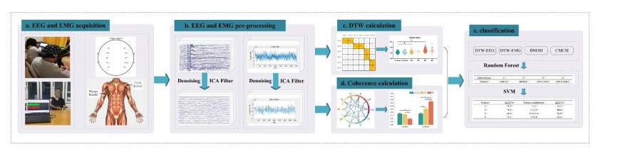
Changes in the functional connections between the cerebral cortex and muscles can evaluate motor function in stroke rehabilitation. To quantify changes in functional connections between the cerebral cortex and muscles, we combined corticomuscular coupling and graph theory to propose dynamic time warped (DTW) distances for electroencephalogram (EEG) and electromyography (EMG) signals as well as two new symmetry metrics. EEG and EMG data from 18 stroke patients and 16 healthy individuals, as well as Brunnstrom scores from stroke patients, were recorded in this paper. First, calculate DTW-EEG, DTW-EMG, BNDSI and CMCSI. Then, the random forest algorithm was used to calculate the feature importance of these biological indicators. Finally, based on the results of feature importance, different features were combined and validated for classification. The results showed that the feature importance was from high to low as CMCSI/BNDSI/DTW-EEG/DTW-EMG, while the feature combination with the highest accuracy was CMCSI+BNDSI+DTW-EEG. Compared to previous studies, combining the CMCSI+BNDSI+DTW-EEG features of EEG and EMG achieved better results in the prediction of motor function rehabilitation at different levels of stroke. Our work implies that the establishment of a symmetry index based on graph theory and cortical muscle coupling has great potential in predicting stroke recovery and promises to have an impact on clinical research applications.

| [1] |
K. Mira, L. Andreas, Global Burden of Stroke, Semin. Neurol., 38 (2018), 208–211. https://doi.org/10.1055/s-0038-1649503 doi: 10.1055/s-0038-1649503

|
| [2] |
P. B. Gorelick, The global burden of stroke: Persistent and disabling, Lancet Neurol., 18 (2019), 417–418. https://doi.org/10.1016/S1474-4422(19)30030-4 doi: 10.1016/S1474-4422(19)30030-4
|
| [3] |
C. Stinear, Prediction of recovery of motor function after stroke, Lancet Neurol., 9 (2010), 1228–1232. https://doi.org/10.1016/S1474-4422(10)70247-7 doi: 10.1016/S1474-4422(10)70247-7
|
| [4] |
P. M. Rossini, C. Altamura, A. Ferretti, F. Vernieri, F. Zappasodi, M. Caulo, et al., Does cerebrovascular disease affect the coupling between neuronal activity and local haemodynamics?, Brain, 127 (2004), 99–110. https://doi.org/10.1093/brain/awh012 doi: 10.1093/brain/awh012
|
| [5] |
B. A. Cohen, E. J. Bravo-Fernandez, A. Sances, Quantification of computer analyzed serial EEGs from stroke patients, Electr. Clin. Neurophysiol., 41 (1976), 379–386. https://doi.org/10.1016/0013-4694(76)90100-0 doi: 10.1016/0013-4694(76)90100-0
|
| [6] |
L. Murri, S. Gori, R. Massetani, E. Bonanni, F. Marcella, S. Milani, Evaluation of acute ischemic stroke using quantitative EEG: A comparison with conventional EEG and CT scan, Neurophysiol. Clin./Clin. Neurophysiol., 28 (1998), 249–257. https://doi.org/10.1016/S0987-7053(98)80115-9 doi: 10.1016/S0987-7053(98)80115-9
|
| [7] |
S. P. Finnigan, M. Walsh, S. E. Rose, J. B. Chalk, Quantitative EEG indices of sub-acute ischaemic stroke correlate with clinical outcomes, Clin. Neurophysiol., 118 (2007), 2525–2532. https://doi.org/10.1016/j.clinph.2007.07.021 doi: 10.1016/j.clinph.2007.07.021
|
| [8] |
S. Finnigan, M. J. A. M. van Putten, EEG in ischaemic stroke: quantitative EEG can uniquely inform (sub-)acute prognoses and clinical management, Clin. Neurophysiol., 124 (2013), 10–19. https://doi.org/10.1016/j.clinph.2012.07.003 doi: 10.1016/j.clinph.2012.07.003
|
| [9] |
S. Graziadio, L. Tomasevic, G. Assenza, F. Tecchio, J. A. Eyre, The myth of the 'unaffected' side after unilateral stroke: Is reorganisation of the non-infarcted corticospinal system to re-establish balance the price for recovery?, Exp. Neurol., 238 (2012), 168–175. https://doi.org/10.1016/j.expneurol.2012.08.031 doi: 10.1016/j.expneurol.2012.08.031
|
| [10] |
P. Manganotti, S. Patuzzo, F. Cortese, A. Palermo, N. Smania, A. Fiaschi, Motor disinhibition in affected and unaffected hemisphere in the early period of recovery after stroke, Clin. Neurophysiol., 113 (2002), 936–43. https://doi.org/10.1016/S1388-2457(02)00062-7 doi: 10.1016/S1388-2457(02)00062-7
|
| [11] |
C. Bentes, A. R. Peralta, P. Viana, H. Martins, C. Morgado, C. Casimiro, et al., Quantitative EEG and functional outcome following acute ischemic stroke, Clin. Neurophysiol., 129 (2018), 1680–1687. https://doi.org/10.1016/j.clinph.2018.05.021 doi: 10.1016/j.clinph.2018.05.021
|
| [12] |
M. S. Romagosa, E. Udina, R. Ortner, J. Dinarès-Ferran, W. Cho, N. Murovec, et al., EEG biomarkers related with the functional state of stroke patients, Front. Neurosci., 16 (2022), 1032959. https://doi.org/10.3389/fnins.2022.1032959 doi: 10.3389/fnins.2022.1032959
|
| [13] |
M. Saes, C.G.M. Meskers, A. Daffertshofer, J.C. de Munck, G. Kwakkel, E. E. H. van Wegen, How does upper extremity Fugl-Meyer motor score relate to resting-state EEG in chronic stroke? A power spectral density analysis, Clin. Neurophysiol., 130 (2019), 856–862. https://doi.org/10.1016/j.clinph.2019.01.007 doi: 10.1016/j.clinph.2019.01.007
|
| [14] | B. A. Conway, D. M. Halliday, U. Shahani, P. Maas, A. I. Weir, J. R. Rosenberg, et al., Common frequency components identified from correlations between magnetic recordings of cortical activity and the electromyogram in man, J. Physiol. London, 483 (1995), 35. |
| [15] |
T. Mima, K. Toma, B. Koshy, M. Hallett, Coherence between cortical and muscular activities after subcortical stroke, Stroke, 32 (2001), 2597–601. https://doi.org/10.1161/hs1101.098764 doi: 10.1161/hs1101.098764
|
| [16] |
S. H. Strogatz, Exploring complex networks, Nature, 410 (2001), 268–76. https://doi.org/10.1038/35065725 doi: 10.1038/35065725
|
| [17] |
M. Y. Wang, F. M. Lu, Z. H. Hu, J. Zhang, Z. Yuan, Optical mapping of prefrontal brain connectivity and activation during emotion anticipation, Behav. Brain Res., 350 (2018), 122–128. https://doi.org/10.1016/j.bbr.2018.04.051 doi: 10.1016/j.bbr.2018.04.051
|
| [18] |
J. M. Sheffield, S. Kandala, C. A. Tamminga, G. D. Pearlson, M. S. Keshavan, J. A. Sweeney, et al., Transdiagnostic associations between functional brain network integrity and cognition, JAMA Psychiatry, 74 (2017), 605–613. https://doi.org/10.1001/jamapsychiatry.2017.0669 doi: 10.1001/jamapsychiatry.2017.0669
|
| [19] |
A. K. Andrea, B. Misic, O. Sporns, Communication dynamics in complex brain networks, Nat. Rev. Neurosci., 19 (2017), 17–33. https://doi.org/10.1038/nrn.2017.149 doi: 10.1038/nrn.2017.149
|
| [20] |
F. D. V. Fallani, F. Pichiorri, G. Morone, M. Molinari, F. Babiloni, F. Cincotti, et al., Multiscale topological properties of functional brain networks during motor imagery after stroke, Neuroimage, 83 (2013), 438–49. https://doi.org/10.1016/j.neuroimage.2013.06.039 doi: 10.1016/j.neuroimage.2013.06.039
|
| [21] |
F. Vecchio, C. Tomino, F. Miraglia, F. Iodice, C. Erra, I. R. Di, et al., Cortical connectivity from EEG data in acute stroke: A study via graph theory as a potential biomarker for functional recovery, Int. J. Psychophysiol., 146 (2019), 133–138. https://doi.org/10.1016/j.ijpsycho.2019.09.012 doi: 10.1016/j.ijpsycho.2019.09.012
|
| [22] |
X. L. Chen, P. Xie, Y. Y. Zhang, Y. L. Chen, S. G. Cheng, L. T. Zhang, Abnormal functional corticomuscular coupling after stroke, Neuroimage Clin., 19 (2018), 147–159. https://doi.org/10.1016/j.nicl.2018.04.004 doi: 10.1016/j.nicl.2018.04.004
|
| [23] |
A. Delorme, S. Makeig, EEGLAB: an open source toolbox for analysis of single-trial EEG dynamics including independent component analysis, J. Neurosci. Methods, 134 (2004), 9–21. https://doi.org/10.1016/j.jneumeth.2003.10.009 doi: 10.1016/j.jneumeth.2003.10.009
|
| [24] | T. Mullen, NITRC: CleanLine: Tool/Resource Info, (2012). |
| [25] |
R. Mahajan, B. I.Morshed, Unsupervised eye blink artifact denoising of EEG data with modified multiscale sample entropy, Kurtosis, and wavelet-ICA, IEEE J. Biomed. Health Inf., 19 (2015), 158–65. https://doi.org/10.1109/JBHI.2014.2333010 doi: 10.1109/JBHI.2014.2333010
|
| [26] |
Z. Y. Sun, X. G. Xi, C. M. Yuan, Y. Yang, X. Hua, Surface electromyography signal denoising via EEMD and improved wavelet thresholds, Math. Biosci. Eng., 17 (2020), 6945–6962. https://doi.org/10.3934/mbe.2020359 doi: 10.3934/mbe.2020359
|
| [27] |
H. Liu, W. Wang, C. Xiang, L. Han, H. Nie, A de-noising method using the improved wavelet threshold function based on noise variance estimation, Mech. Syst. Signal Process., 99 (2018), 30–46. https://doi.org/10.1016/j.ymssp.2017.05.034 doi: 10.1016/j.ymssp.2017.05.034
|
| [28] |
D. L. Donoho, I. Johnstone, G. Kerkyacharian, D. Picard, Density estimation by wavelet thresholding, Ann. Stat., 24 (1996), 508–539. https://doi.org/10.1214/aos/1032894451 doi: 10.1214/aos/1032894451
|
| [29] |
K. Robert, L. Enochson, Digital Time Series Analysis, J. Dyn. Sys. Meas. Control, 95 (1973), 442. https://doi.org/10.1115/1.3426753 doi: 10.1115/1.3426753
|
| [30] |
M. J. A. M. van Putten, D. L. J. Tavy, Continuous quantitative EEG monitoring in hemispheric stroke patients using the brain symmetry index, Stroke, 35 (2004), 2489–92. https://doi.org/10.1161/01.STR.0000144649.49861.1d doi: 10.1161/01.STR.0000144649.49861.1d
|
| [31] |
M. Molnár, R. Csuhaj, S. Horváth, L. Vastsgh, Z. A. Gaál, B. Czigler, Spectral and complexity features of the EEG changed by visual input in a case of subcortical stroke compared to healthy controls, Clin. Neurophysiol., 117 (2006), 771–780. https://doi.org/10.1016/j.clinph.2005.12.022 doi: 10.1016/j.clinph.2005.12.022
|
| [32] |
B. H. Menze, B. M. Kelm, R. Masuch, U. Himmelreich, P. Bachert, W. Petrich, et al., A comparison of random forest and its Gini importance with standard chemometric methods for the feature selection and classification of spectral data, BMC Bioinf., 10 (2009), 213. https://doi.org/10.1186/1471-2105-10-213 doi: 10.1186/1471-2105-10-213
|
| [33] |
C. Cortes, V. Vapnik, Support vector machine, Mach. Learn., 20 (1995), 273–297. https://doi.org/10.1007/BF00994018 doi: 10.1007/BF00994018
|
| [34] | E. W. Guntari, E. C. Djamal, F. Nugraha, S. L. L. Liem, Classification of post-stroke EEG signal using genetic algorithm and recurrent neural networks, in 2020 7th International Conference on Electrical Engineering, Computer Sciences and Informatics (EECSI), IEEE, 12 (2020), 156–161. https://doi.org/10.23919/EECSI50503.2020.9251296 |
| [35] |
N. Vivaldi, M. Caiola, K. Solarana, M. Ye, Evaluating Performance of EEG data-driven machine learning for traumatic brain injury classification, IEEE Trans. Biomed. Eng., 68 (2021), 3205–3216. https://doi.org/10.1109/TBME.2021.3062502 doi: 10.1109/TBME.2021.3062502
|
| [36] | A. U. Fadiyah, E. C. Djamal, Classification of motor imagery and synchronization of post-stroke patient EEG signal, in 2019 6th International Conference on Electrical Engineering, Computer Science and Informatics (EECSI), IEEE, 3 (2019), 28–33. https://doi.org/10.23919/EECSI48112.2019.8977076 |
| [37] |
X. G. Xi, S. J. Pi, Y. B. Zhao, H. J. Wang, Z. Z. Luo, Effect of muscle fatigue on the cortical-muscle network: A combined electroencephalogram and electromyogram study, Brain Res., 1752 (2021), 147221. https://doi.org/10.1016/j.brainres.2020.147221 doi: 10.1016/j.brainres.2020.147221
|
| [38] |
S. Angelova, S. Ribagin, R. Raikova, I. Veneva, Power frequency spectrum analysis of surface EMG signals of upper limb muscles during elbow flexion–A comparison between healthy subjects and stroke survivors, J. Electromyogr. Kinesiology, 38 (2018), 7–16. https://doi.org/10.1016/j.jelekin.2017.10.013 doi: 10.1016/j.jelekin.2017.10.013
|
| [39] |
R. Kawashima, K. Yamada, S. Kinomura, T. Yamaguchi, H. Matsui, S. Yoshioka, et al., Regional cerebral blood flow changes of cortical motor areas and prefrontal areas in humans related to ipsilateral and contralateral hand movement, Brain Res., 623 (1993), 33–40. https://doi.org/10.1016/0006-8993(93)90006-9 doi: 10.1016/0006-8993(93)90006-9
|
| [40] |
A. A. Agius, O. Falzon, K. Camilleri, M. Vella, R. Muscat, Brain symmetry index in healthy and stroke patients for assessment and prognosis, Stroke Res. Treat., 2017 (2017), 9. https://doi.org/10.1155/2017/8276136 doi: 10.1155/2017/8276136
|
| [41] |
L. L. H. Pan, W. W. Yang, C. L. Kao, M. W. Tsai, S. H. Wei, F. Fregni, et al., Effects of 8-week sensory electrical stimulation combined with motor training on EEG-EMG coherence and motor function in individuals with stroke, Sci. Rep., 8 (2018), 9217. https://doi.org/10.1038/s41598-018-27553-4 doi: 10.1038/s41598-018-27553-4
|
| [42] |
V. Svetnik, A. Liaw, C. Tong, J. C. Culberson, R. P. Sheridan, B. P. Feuston, Random forest: A classification and regression tool for compound classification and QSAR modeling, J. Chem. Inf. Comput. Sci., 43 (2003), 1947–58. https://doi.org/10.1021/ci034160g doi: 10.1021/ci034160g
|
| [43] |
J. Rogers, S. Middleton, P. H. Wilson, S. J. Johnstone, Predicting functional outcomes after stroke: An observational study of acute single-channel EEG, Top. Stroke Rehabil., 27 (2020), 161–172. https://doi.org/10.1080/10749357.2019.1673576 doi: 10.1080/10749357.2019.1673576
|
| [44] |
R. J. Zhou, H. M. Hondori, M. Khademi, J. M. Cassidy, K. M. Wu, D. Z. Yang, et al., Predicting gains with visuospatial training after stroke using an EEG measure of frontoparietal circuit function, Front. Neurol., 9 (2018), 597. https://doi.org/10.3389/fneur.2018.00597 doi: 10.3389/fneur.2018.00597
|
| [45] |
Y. Celik, S. Stuart, W. L. Woo, E. Sejdic, A. Godfrey, Multi-modal gait: A wearable, algorithm and data fusion approach for clinical and free-living assessment, Inf. Fusion, 78 (2022), 57–70. https://doi.org/10.1016/j.inffus.2021.09.016 doi: 10.1016/j.inffus.2021.09.016
|
| [46] |
S. Qiu, H. Zhao, N. Jiang, Z. Wang, L. Liu, Y. An, et al., Multi-sensor information fusion based on machine learning for real applications in human activity recognition: State-of-the-art and research challenges, Inf. Fusion, 80 (2022), 241–265. https://doi.org/10.1016/j.inffus.2021.11.006 doi: 10.1016/j.inffus.2021.11.006
|
| [47] |
A. Talitckii, E. Kovalenko, A. Shcherbak, A. Anikina, E. Bril, O. Zimniakova, et al., Comparative study of wearable sensors, video, and handwriting to detect Parkinson's disease, IEEE Trans. Instrumentation Measurement, 71 (2022), 1–10. https://doi.org/10.1109/TIM.2022.3176898 doi: 10.1109/TIM.2022.3176898
|


Figures(7) / Tables(7)

Xian Hua, Jing Li, Ting Wang, Junhong Wang, Shaojun Pi, Hangcheng Li, Xugang Xi. Evaluation of movement functional rehabilitation after stroke: A study via graph theory and corticomuscular coupling as potential biomarker[J]. Mathematical Biosciences and Engineering, 2023, 20(6): 10530-10551. doi: 10.3934/mbe.2023465


 DownLoad: