The 5-methylcytosine (5mC) in the promoter region plays a significant role in biological processes and diseases. A few high-throughput sequencing technologies and traditional machine learning algorithms are often used by researchers to detect 5mC modification sites. However, high-throughput identification is laborious, time-consuming and expensive; moreover, the machine learning algorithms are not so advanced. Therefore, there is an urgent need to develop a more efficient computational approach to replace those traditional methods. Since deep learning algorithms are more popular and have powerful computational advantages, we constructed a novel prediction model, called DGA-5mC, to identify 5mC modification sites in promoter regions by using a deep learning algorithm based on an improved densely connected convolutional network (DenseNet) and the bidirectional GRU approach. Furthermore, we added a self-attention module to evaluate the importance of various 5mC features. The deep learning-based DGA-5mC model algorithm automatically handles large proportions of unbalanced data for both positive and negative samples, highlighting the model's reliability and superiority. So far as the authors are aware, this is the first time that the combination of an improved DenseNet and bidirectional GRU methods has been used to predict the 5mC modification sites in promoter regions. It can be seen that the DGA-5mC model, after using a combination of one-hot coding, nucleotide chemical property coding and nucleotide density coding, performed well in terms of sensitivity, specificity, accuracy, the Matthews correlation coefficient (MCC), area under the curve and Gmean in the independent test dataset: 90.19%, 92.74%, 92.54%, 64.64%, 96.43% and 91.46%, respectively. In addition, all datasets and source codes for the DGA-5mC model are freely accessible at https://github.com/lulukoss/DGA-5mC.
Citation: Jianhua Jia, Lulu Qin, Rufeng Lei. DGA-5mC: A 5-methylcytosine site prediction model based on an improved DenseNet and bidirectional GRU method[J]. Mathematical Biosciences and Engineering, 2023, 20(6): 9759-9780. doi: 10.3934/mbe.2023428
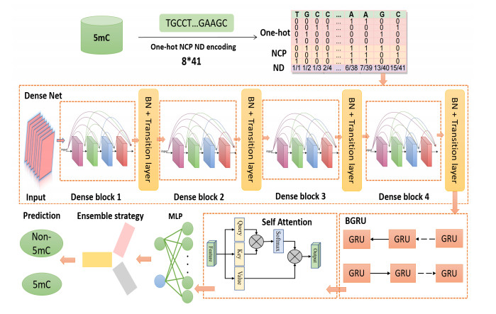
The 5-methylcytosine (5mC) in the promoter region plays a significant role in biological processes and diseases. A few high-throughput sequencing technologies and traditional machine learning algorithms are often used by researchers to detect 5mC modification sites. However, high-throughput identification is laborious, time-consuming and expensive; moreover, the machine learning algorithms are not so advanced. Therefore, there is an urgent need to develop a more efficient computational approach to replace those traditional methods. Since deep learning algorithms are more popular and have powerful computational advantages, we constructed a novel prediction model, called DGA-5mC, to identify 5mC modification sites in promoter regions by using a deep learning algorithm based on an improved densely connected convolutional network (DenseNet) and the bidirectional GRU approach. Furthermore, we added a self-attention module to evaluate the importance of various 5mC features. The deep learning-based DGA-5mC model algorithm automatically handles large proportions of unbalanced data for both positive and negative samples, highlighting the model's reliability and superiority. So far as the authors are aware, this is the first time that the combination of an improved DenseNet and bidirectional GRU methods has been used to predict the 5mC modification sites in promoter regions. It can be seen that the DGA-5mC model, after using a combination of one-hot coding, nucleotide chemical property coding and nucleotide density coding, performed well in terms of sensitivity, specificity, accuracy, the Matthews correlation coefficient (MCC), area under the curve and Gmean in the independent test dataset: 90.19%, 92.74%, 92.54%, 64.64%, 96.43% and 91.46%, respectively. In addition, all datasets and source codes for the DGA-5mC model are freely accessible at https://github.com/lulukoss/DGA-5mC.

| [1] |
Y. Assenov, F. Muller, P. Lutsik, J. Walter, T. Lengauer, C. Bock, Comprehensive analysis of DNA methylation data with RnBeads, Nat. Methods, 11 (2014), 1138–1140. https://doi.org/10.1038/nmeth.3115 doi: 10.1038/nmeth.3115

|
| [2] |
M. Beetch, C. Boycott, S. Harandi-Zadeh, T. Yang, B. J. E. Martin, T. Dixon-McDougall, et al., Pterostilbene leads to DNMT3B-mediated DNA methylation and silencing of OCT1-targeted oncogenes in breast cancer cells, J. Nutr. Biochem., 98 (2021), 108815. https://doi.org/10.1016/j.jnutbio.2021.108815 doi: 10.1016/j.jnutbio.2021.108815
|
| [3] |
H. Lv, F. Y. Dao, D. Zhang, H. Yang, H. Lin, Advances in mapping the epigenetic modifications of 5-methylcytosine (5mC), N6-methyladenine (6mA), and N4-methylcytosine (4mC), Biotechnol. Bioeng., 118 (2021), 4204–4216. https://doi.org/10.1002/bit.27911 doi: 10.1002/bit.27911
|
| [4] |
J. Karanthamalai, A. Chodon, S. Chauhan, G. Pandi, DNA N6-methyladenine modification in plant genomes-A glimpse into emerging epigenetic code, Plants, 9 (2020). https://doi.org/10.3390/plants9020247 doi: 10.3390/plants9020247
|
| [5] |
J. Xiong, K. K. Chen, N. B. Xie, T. T. Ji, S. Y. Yu, F. Tang, et al., Bisulfite-free and single-base resolution detection of epigenetic DNA modification of 5-Methylcytosine by methyltransferase-directed labeling with APOBEC3A deamination sequencing, Anal. Chem., 94 (2022), 15489–15498. https://doi.org/10.1021/acs.analchem.2c03808 doi: 10.1021/acs.analchem.2c03808
|
| [6] |
Q. Zhang, Y. Wu, Q. Xu, F. Ma, C. Y. Zhang, Recent advances in biosensors for in vitro detection and in vivo imaging of DNA methylation, Biosens. Bioelectron., 171 (2021), 112712. https://doi.org/10.1016/j.bios.2020.112712 doi: 10.1016/j.bios.2020.112712
|
| [7] |
D. K. Vanaja, M. Ehrich, D. Van den Boom, J. C. Cheville, R. J. Karnes, D. J. Tindall, et al., Hypermethylation of genes for diagnosis and risk stratification of prostate cancer, Cancer Invest., 27 (2009), 549–560. https://doi.org/10.1080/07357900802620794 doi: 10.1080/07357900802620794
|
| [8] |
K. Chen, J. Zhang, Z. Guo, Q. Ma, Z. Xu, Y. Zhou, et al., Loss of 5-hydroxymethylcytosine is linked to gene body hypermethylation in kidney cancer, Cell Res., 26 (2016), 103–118. https://doi.org/10.1038/cr.2015.150 doi: 10.1038/cr.2015.150
|
| [9] |
D. W. Tucker, C. R. Getchell, E. T. McCarthy, A. W. Ohman, N. Sasamoto, S. Xu, et al., Epigenetic reprogramming strategies to reverse global loss of 5-Hydroxymethylcytosine, a prognostic factor for poor survival in high-grade serous ovarian cancer, Clin. Cancer Res., 24 (2018), 1389–1401. https://doi.org/10.1158/1078-0432.CCR-17-1958 doi: 10.1158/1078-0432.CCR-17-1958
|
| [10] |
P. Devi, S. Ota, T. Punga, A. Bergqvist, Hepatitis C virus core protein down-regulates expression of src-homology 2 domain containing protein tyrosine phosphatase by modulating promoter DNA methylation, Viruses, 13 (2021). https://doi.org/10.3390/v13122514 doi: 10.3390/v13122514
|
| [11] |
J. Rodriguez-Ubreva, C. de la Calle-Fabregat, T. Li, L. Ciudad, M. L. Ballestar, F. Catala-Moll, et al., Inflammatory cytokines shape a changing DNA methylome in monocytes mirroring disease activity in rheumatoid arthritis, Ann. Rheum. Dis., 78 (2019), 1505–1516. https://doi.org/10.1136/annrheumdis-2019-215355 doi: 10.1136/annrheumdis-2019-215355
|
| [12] |
L. Wei, R. Su, S. Luan, Z. Liao, B. Manavalan, Q. Zou, et al., Iterative feature representations improve N4-methylcytosine site prediction, Bioinformatics, 35 (2019), 4930–4937. https://doi.org/10.1093/bioinformatics/btz408 doi: 10.1093/bioinformatics/btz408
|
| [13] |
S. Shinagawa, N. Kobayashi, T. Nagata, A. Kusaka, H. Yamada, K. Kondo, et al., DNA methylation in the NCAPH2/LMF2 promoter region is associated with hippocampal atrophy in Alzheimer's disease and amnesic mild cognitive impairment patients, Neurosci. Lett., 629 (2016), 33–37. https://doi.org/10.1016/j.neulet.2016.06.055 doi: 10.1016/j.neulet.2016.06.055
|
| [14] |
L. Zhang, Y. Z. Xu, X. F. Xiao, J. Chen, X. Q. Zhou, W. Y. Zhu, et al., Development of techniques for DNA-methylation analysis, TrAC, Trends Anal. Chem., 72 (2015), 114–122. https://doi.org/10.1016/j.trac.2015.03.025 doi: 10.1016/j.trac.2015.03.025
|
| [15] |
M. Lecorguille, F. M. McAuliffe, P. J. Twomey, K. Viljoen, J. Mehegan, C. C. Kelleher, et al., Maternal glycaemic and insulinemic status and newborn DNA methylation: findings in women with overweight and obesity, J. Clin. Endocrinol. Metab., 108 (2023), 85–98. https://doi.org/10.1210/clinem/dgac553 doi: 10.1210/clinem/dgac553
|
| [16] |
X. Su, Y. Chu, J. H. Kordower, B. Li, H. Cao, L. Huang, et al., PGC-1α promoter methylation in Parkinson's disease, PLoS One, 10 (2015), e0134087. https://doi.org/10.1371/journal.pone.0134087 doi: 10.1371/journal.pone.0134087
|
| [17] |
L. Yang, Y. Chen, N. Liu, Y. Lu, X. Li, W. Ma, et al., 5mC and H3K9me3 of TRAF3IP2 promoter region accelerates the progression of translocation renal cell carcinoma, Biomarker Res., 10 (2022). https://doi.org/10.1186/s40364-022-00402-3 doi: 10.1186/s40364-022-00402-3
|
| [18] |
F. Nassiri, A. Chakravarthy, S. Feng, S. Y. Shen, R. Nejad, J. A. Zuccato, et al., Detection and discrimination of intracranial tumors using plasma cell-free DNA methylomes, Nat. Med., 26 (2020), 1044–1047. https://doi.org/10.1038/s41591-020-0932-2 doi: 10.1038/s41591-020-0932-2
|
| [19] |
M. J. Booth, T. W. Ost, D. Beraldi, N. M. Bell, M. R. Branco, W. Reik, et al., Oxidative bisulfite sequencing of 5-methylcytosine and 5-hydroxymethylcytosine, Nat. Protoc., 8 (2013), 1841–1851. https://doi.org/10.1038/nprot.2013.115 doi: 10.1038/nprot.2013.115
|
| [20] | Y. Li, T. O. Tollefsbol, DNA methylation detection: bisulfite genomic sequencing analysis, in Epigenetics Protocols, Humana Press, 791 (2011), 11–21. https://doi.org/10.1007/978-1-61779-316-5_2 |
| [21] |
D. Chai, C. Jia, J. Zheng, Q. Zou, F. Li, Staem5: A novel computational approachfor accurate prediction of m5C site, Mol. Ther. Nucleic Acids, 26 (2021), 1027–1034. https://doi.org/10.1016/j.omtn.2021.10.012 doi: 10.1016/j.omtn.2021.10.012
|
| [22] |
Y. Liu, Y. Shen, H. Wang, Y. Zhang, X. Zhu, m5Cpred-XS: A new method for predicting RNA m5C sites based on XGBoost and SHAP, Front. Genet., 13 (2022). https://doi.org/10.3389/fgene.2022.853258 doi: 10.3389/fgene.2022.853258
|
| [23] |
X. Chen, Y. Xiong, Y. Liu, Y. Chen, S. Bi, X. Zhu, m5CPred-SVM: a novel method for predicting m5C sites of RNA, BMC Bioinf., 21 (2020). https://doi.org/10.1186/s12859-020-03828-4 doi: 10.1186/s12859-020-03828-4
|
| [24] |
M. M. Hasan, S. Tsukiyama, J. Y. Cho, H. Kurata, M. A. Alam, X. Liu, et al., Deepm5C: A deep-learning-based hybrid framework for identifying human RNA N5-methylcytosine sites using a stacking strategy, Mol. Ther., 30 (2022), 2856–2867. https://doi.org/10.1016/j.ymthe.2022.05.001 doi: 10.1016/j.ymthe.2022.05.001
|
| [25] |
H. Shi, S. Zhang, X. Li, R5hmCFDV: computational identification of RNA 5-hydroxymethylcytosine based on deep feature fusion and deep voting, Briefings Bioinf., 23 (2022). https://doi.org/10.1093/bib/bbac341 doi: 10.1093/bib/bbac341
|
| [26] |
H. Wang, S. Wang, Y. Zhang, S. Bi, X. Zhu, A brief review of machine learning methods for RNA methylation sites prediction, Methods, 203 (2022), 399–421. https://doi.org/10.1016/j.ymeth.2022.03.001 doi: 10.1016/j.ymeth.2022.03.001
|
| [27] |
G. Guo, K. Pan, S. Fang, L. Ye, X. Tong, Z. Wang, et al., Advances in mRNA 5-methylcytosine modifications: Detection, effectors, biological functions, and clinical relevance, Mol. Ther. Nucleic Acids, 26 (2021), 575–593. https://doi.org/10.1016/j.omtn.2021.08.020 doi: 10.1016/j.omtn.2021.08.020
|
| [28] |
A. El Allali, Z. Elhamraoui, R. Daoud, Machine learning applications in RNA modification sites prediction, Comput. Struct. Biotechnol. J., 19 (2021), 5510–5524. https://doi.org/10.1016/j.csbj.2021.09.025 doi: 10.1016/j.csbj.2021.09.025
|
| [29] |
L. Zhang, X. Xiao, Z. C. Xu, iPromoter-5mC: A novel fusion decision predictor for the identification of 5-Methylcytosine sites in genome-wide DNA promoters, Front. Cell Dev. Biol., 8 (2020). https://doi.org/10.3389/fcell.2020.00614 doi: 10.3389/fcell.2020.00614
|
| [30] |
L. Fu, B. Niu, Z. Zhu, S. Wu, W. Li, CD-HIT: accelerated for clustering the next-generation sequencing data, Bioinformatics, 28 (2012), 3150–3152. https://doi.org/10.1093/bioinformatics/bts565 doi: 10.1093/bioinformatics/bts565
|
| [31] |
T. T. Nguyen, T. A. Tran, N. Q. Le, D. M. Pham, Y. Y. Ou, An extensive examination of discovering 5-Methylcytosine sites in genome-wide DNA promoters using machine learning based approaches, IEEE/ACM Trans. Comput. Biol. Bioinf., 19 (2022), 87–94. https://doi.org/10.1109/TCBB.2021.3082184 doi: 10.1109/TCBB.2021.3082184
|
| [32] |
W. R. Qiu, X. Xiao, Y. T. Shao, Z. T. Luo, m5C-HPromoter: An ensemble deep learning predictor for identifying 5-methylcytosine sites in human promoters, Curr. Bioinf., 17 (2022), 452–461. https://doi.org/10.2174/1574893617666220330150259 doi: 10.2174/1574893617666220330150259
|
| [33] |
X. Cheng, J. Wang, Q. Li, T. Liu, BiLSTM-5mC: A bidirectional long short-term memory-based approach for predicting 5-Methylcytosine sites in genome-wide DNA promoters, Molecules, 26 (2021). https://doi.org/10.3390/molecules26247414 doi: 10.3390/molecules26247414
|
| [34] |
H. Wang, Z. Yan, D. Liu, H. Zhao, J. Zhao, MDC-Kace: A model for predicting Lysine acetylation sites based on modular densely Connected Convolutional Networks, IEEE Access, 8 (2020), 214469–214480. https://doi.org/10.1109/access.2020.3041044 doi: 10.1109/access.2020.3041044
|
| [35] |
J. Jia, G. Wu, M. Li, W. Qiu, pSuc-EDBAM: Predicting lysine succinylation sites in proteins based on ensemble dense blocks and an attention module, BMC Bioinf., 23 (2022), 450. https://doi.org/10.1186/s12859-022-05001-5 doi: 10.1186/s12859-022-05001-5
|
| [36] |
J. Jia, M. Sun, G. Wu, W. Qiu, DeepDN_iGlu: prediction of lysine glutarylation sites based on attention residual learning method and DenseNet, Math. Biosci. Eng., 20 (2022), 2815–2830. https://doi.org/10.3934/mbe.2023132 doi: 10.3934/mbe.2023132
|
| [37] |
X. Li, S. Zhang, H. Shi, An improved residual network using deep fusion for identifying RNA 5-methylcytosine sites, Bioinformatics, 38 (2022), 4271–4277. https://doi.org/10.1093/bioinformatics/btac532 doi: 10.1093/bioinformatics/btac532
|
| [38] |
S. Min, B. Lee, S. Yoon, Deep learning in bioinformatics, Briefings Bioinf., 18 (2017), 851–869. https://doi.org/10.1093/bib/bbw068 doi: 10.1093/bib/bbw068
|
| [39] |
J. Jin, Y. Yu, L. Wei, Mouse4mC-BGRU: Deep learning for predicting DNA N4-methylcytosine sites in mouse genome, Methods, 204 (2022), 258–262. https://doi.org/10.1016/j.ymeth.2022.01.009 doi: 10.1016/j.ymeth.2022.01.009
|
| [40] |
Q. Ning, J. Li, DLF-Sul: a multi-module deep learning framework for prediction of S-sulfinylation sites in proteins, Briefings Bioinf., 23 (2022). https://doi.org/10.1093/bib/bbac323 doi: 10.1093/bib/bbac323
|
| [41] |
Z. Y. Zhang, L. Ning, X. Ye, Y. H. Yang, Y. Futamura, T. Sakurai, et al., iLoc-miRNA: extracellular/intracellular miRNA prediction using deep BiLSTM with attention mechanism, Briefings Bioinf., 23 (2022). https://doi.org/10.1093/bib/bbac395 doi: 10.1093/bib/bbac395
|
| [42] |
Z. Luo, W. Su, L. Lou, W. Qiu, X. Xiao, Z. Xu, DLm6Am: A Deep-Learning-Based Tool for Identifying N6, 2'-O-Dimethyladenosine Sites in RNA Sequences, Int. J. Mol. Sci., 23 (2022). https://doi.org/10.3390/ijms231911026 doi: 10.3390/ijms231911026
|
| [43] |
H. Li, S. Ning, M. Ghandi, G. V. Kryukov, S. Gopal, A. Deik, et al., The landscape of cancer cell line metabolism, Nat. Med., 25 (2019), 850–860. https://doi.org/10.1038/s41591-019-0404-8 doi: 10.1038/s41591-019-0404-8
|
| [44] |
T. H. Nguyen-Vo, Q. H. Nguyen, T. T. T. Do, T. N. Nguyen, S. Rahardja, B. P. Nguyen, iPseU-NCP: Identifying RNA pseudouridine sites using random forest and NCP-encoded features, BMC Genomics., 20 (2019), 971. https://doi.org/10.1186/s12864-019-6357-y doi: 10.1186/s12864-019-6357-y
|
| [45] |
Z. Cui, L. Kang, L. Li, L. Wang, K. Wang, A combined state-of-charge estimation method for lithium-ion battery using an improved BGRU network and UKF, Energy, 259 (2022). https://doi.org/10.1016/j.energy.2022.124933 doi: 10.1016/j.energy.2022.124933
|
| [46] |
Y. Shang, X. Tang, G. Zhao, P. Jiang, T. Ran Lin, A remaining life prediction of rolling element bearings based on a bidirectional gate recurrent unit and convolution neural network, Measurement, 202 (2022). https://doi.org/10.1016/j.measurement.2022.111893 doi: 10.1016/j.measurement.2022.111893
|
| [47] |
S. Yang, G. Berdine, The receiver operating characteristic (ROC) curve, Southwest Respir. Crit. Care Chron., 5 (2017), 34–36. https://doi.org/10.12746/swrccc.v5i19.391 doi: 10.12746/swrccc.v5i19.391
|


Figures(12) / Tables(8)

Jianhua Jia, Lulu Qin, Rufeng Lei. DGA-5mC: A 5-methylcytosine site prediction model based on an improved DenseNet and bidirectional GRU method[J]. Mathematical Biosciences and Engineering, 2023, 20(6): 9759-9780. doi: 10.3934/mbe.2023428


 DownLoad: