Excess mortality and COVID-19 deaths in Italy: A peak comparison study

Marco Roccetti; Marco Roccetti

doi:10.3934/mbe.2023304

Mathematical Biosciences and Engineering

2023, Volume 20, Issue 4: 7042-7055. doi: 10.3934/mbe.2023304

Previous Article Next Article

Research article Special Issues

Excess mortality and COVID-19 deaths in Italy: A peak comparison study

Marco Roccetti ^,

Department of Computer Science and Engineering, University of Bologna, Bologna, Italy

Academic Editor: Pierre Magal

Received: 24 December 2022 Revised: 05 February 2023 Accepted: 06 February 2023 Published: 09 February 2023

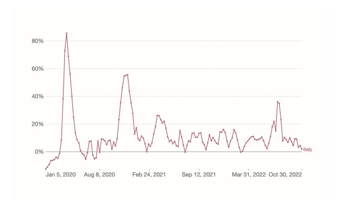
During a sanitary crisis, excess mortality measures the number of all-cause deaths, beyond what we would have expected if that crisis had not occurred. The high number of COVID-19 deaths started a debate in Italy with two opposite positions: those convinced that COVID-19 deaths were not by default excess deaths, because many COVID-19 deaths were not correctly registered, with most being attributable to other causes and to the overall crisis conditions; and those who presented the opposite hypothesis. We analyzed the curve of the all-cause excess mortality, during the period of January 5, 2020–October 31, 2022, compared to the curve of the daily confirmed COVID-19 deaths, investigating the association between excess mortality and the recurrence of COVID-19 waves in Italy. We compared the two curves looking for the corresponding highest peaks, and we found that 5 out of the 6 highest peaks (83.3%) of the excess mortality curve have occurred, on average, just a week before the concomitant COVID-19 waves hit their highest peaks of daily deaths (Mean 6.4 days; SD 2.4 days). This temporal correspondence between the moments when the excess mortality peaked and the highest peaks of the COVID-19 deaths, provides further evidence in favor of a positive correlation between COVID-19 deaths and all-cause excess mortality.
- COVID-19,
- pandemic,
- Italy,
- daily confirmed deaths,
- all-cause excess mortality,
- peak comparison,
- public health
Citation: Marco Roccetti. Excess mortality and COVID-19 deaths in Italy: A peak comparison study[J]. Mathematical Biosciences and Engineering, 2023, 20(4): 7042-7055. doi: 10.3934/mbe.2023304

Related Papers:

Abstract

During a sanitary crisis, excess mortality measures the number of all-cause deaths, beyond what we would have expected if that crisis had not occurred. The high number of COVID-19 deaths started a debate in Italy with two opposite positions: those convinced that COVID-19 deaths were not by default excess deaths, because many COVID-19 deaths were not correctly registered, with most being attributable to other causes and to the overall crisis conditions; and those who presented the opposite hypothesis. We analyzed the curve of the all-cause excess mortality, during the period of January 5, 2020–October 31, 2022, compared to the curve of the daily confirmed COVID-19 deaths, investigating the association between excess mortality and the recurrence of COVID-19 waves in Italy. We compared the two curves looking for the corresponding highest peaks, and we found that 5 out of the 6 highest peaks (83.3%) of the excess mortality curve have occurred, on average, just a week before the concomitant COVID-19 waves hit their highest peaks of daily deaths (Mean 6.4 days; SD 2.4 days). This temporal correspondence between the moments when the excess mortality peaked and the highest peaks of the COVID-19 deaths, provides further evidence in favor of a positive correlation between COVID-19 deaths and all-cause excess mortality.

References

[1]	World Health Organization: Coronavirus (COVID-19) Dashboard, 2023 Available from: https://covid19.who.int/.
[2]	World Health Organization: International Guidelines for Certification and Classification (Coding) of COVID-19 as Cause of Death, 2023 Available from: https://www.who.int/publications/m/item/international-guidelines-for-certification-and-classification-(coding)-of-covid-19-as-cause-of-death.
[3]	M. Lewiński, P Abreu, Arguing About "COVID": Metalinguistic arguments on what counts as a "COVID-19 Death", in The Pandemic of Argumentation, Springer, Cham, Switzerland, (2022), 17-41. https://doi.org/10.1007/978-3-030-91017-4_2
[4]	M. C., Amoretti, E. Lalumera, COVID-19 as the underlying cause of death: disentangling facts and values, Hist. Philos. Life Sci., 43 (2021), 1-4. https://doi.org/10.1007/s40656-020-00355-6 doi: 10.1007/s40656-020-00355-6
[5]	B. I. B. Lindahl, COVID-19 and the selection problem in national cause-of-death statistics, Hist. Philos. Life Sci., 43 (2021), 43-72. https://doi.org/10.1007/s40656-021-00420-8 doi: 10.1007/s40656-021-00420-8
[6]	N. Schwalbe, We could be vastly overestimating the death rate for COVID-19. Here's why. World Economic Forum, 2023. Available from: https://www.weforum.org/agenda/2020/04/we-could-be-vastly-overestimating-the-death-rate-for-covid-19-heres-why/
[7]	D. Adam, The pandemic's true death toll: millions more than official counts, Nature, 601 (2022), 312-315. https://doi.org/10.1038/d41586-022-00104-8 doi: 10.1038/d41586-022-00104-8
[8]	P. Jha, Y. Deshmukh, C. Tumbe, W. Suraweera, A. Bhowmick, S. Sharma, et al., COVID mortality in India: National survey data and health facility deaths, Science, 375 (2022), 667-671. https://doi.org/10.1126/science.abm5154 doi: 10.1126/science.abm5154
[9]	L. S. Versteergard, J. Nielsen, L. Richter, D. Schmid, N. Bustos, T. Braeye, et al., Excess all-cause mortality during the COVID-19 pandemic in Europe - preliminary pooled estimates from the EuroMOMO network, March to April 2020, Eurosurveillance, 25 (2020), 1-6. https://doi.org/10.2807/1560-7917.ES.2020.25.26.2001214
[10]	M. Dorucci, G. Minelli, S Boros, V. Manno, S. Prati, M. Battaglini, et al., Excess mortality in Italy during the COVID-19 pandemic: Assessing the differences between the first and the second wave, Year 2020, Front. Public Health, 9 (2020), 1-9. https://doi.org/10.3389/fpubh.2021.669209
[11]	COVID-19 Excess Mortality Collaborators, Estimating excess mortality due to the COVID-19 pandemic: a systematic analysis of COVID-19-related mortality, 2020-21, Lancet, 399 (2022), 1513-1536. https://doi.org/10.1016/S0140-6736(21)02796-3
[12]	World Health Organization: Coronavirus (COVID-19) Dashboard, 2023. Available from: https://covid19.who.int/region/euro/country/it.
[13]	Italian Institute of Statistics: Epidemia COVID-19 in Italia - Anni 2020 - 2021, 2023. Available from: https://www.istat.it/it/files//2022/03/Epidemia-Covid-19_Infografica-accessibile.pdf.
[14]	K. Harmer, G. Howells, W. Sheng, M. Fairhurst, F. Deravi, A Peak-Trough detection algorithm based on momentum, in Proceedings of IEEE 2008 Congress on Image and Signal Processing, (2008), 454-458. https://doi.org/10.1109/CISP.2008.704
[15]	G. K. Palshikar, Simple algorithms for peak detection in time series, in Proceedings of First Conference on Advanced Data Analysis, Business Analytics and Intelligence, 2009.
[16]	E. Mathieu, H. Ritchie, L. Rodés Guirao, C. Appel, D. Gavrilov, C. Giattino, et al., Coronavirus Pandemic (COVID-19), 2023. Available from: https://ourworldindata.org/covid-deaths.
[17]	L. Németh, D. A. Jdanov, V. M. Shkolnikov, An open-sourced, web-based application to analyze weekly excess mortality based on the short-term mortality fluctuations data series, PLoS ONE, 16 (2021). https://doi.org/10.1371/journal.pone.0246663 doi: 10.1371/journal.pone.0246663
[18]	A. Karlinsky, D. Kobak, Tracking excess mortality across countries during the COVID-19 pandemic with the World Mortality Dataset, eLife, 2021, https://doi.org/10.7554/eLife.69336 doi: 10.7554/eLife.69336
[19]	J. Aron, J. Muellbauer, A pandemic primer on excess mortality statistics and their compatibility across countries, 2023. Available from: https://ourworldindata.org/covid-excess-mortality.
[20]	M. Miller, Novel coronavirus COVID-19 (2019-nCoV) data repository, Bull. Assoc. Can. Map Libr. Arch., 164 (2020). https://doi.org/10.15353/acmla.n164.1730 doi: 10.15353/acmla.n164.1730
[21]	R. Cappi, L. Casini, D. Tosi, M. Roccetti, Questioning the seasonality of SARS-COV-2: a Fourier spectral analysis, BMJ Open, 12 (2022), e061602. https://doi.org/10.1136/bmjopen-2022-061602 doi: 10.1136/bmjopen-2022-061602
[22]	S. X. Zhang, F. Arroyo Marioli, R. Gao, S. Wang, A second wave? What do people mean by COVID waves? - a working definition of epidemic waves, Risk Manag. Healthc Policy, 14 (2021), 3775-82. https://doi.org/10.2147/RMHP.S326051 doi: 10.2147/RMHP.S326051
[23]	L. Casini, M. Roccetti, Reopening Italy's schools in September 2020: A Bayesian estimation of the change in the growth rate of new SARS-CoV-2 cases, BMJ Open, 2021. https://doi.org/10.1136/bmjopen-2021-051458 doi: 10.1136/bmjopen-2021-051458
[24]	L. Modenese, T. Loney, F. Gobba, COVID-19-related mortality amongst physicians in Italy: Trend pre- and post-SARS-CoV-2 vaccination campaign, Healthcare, 10 (2022). https://doi.org/10.3390/healthcare10071187 doi: 10.3390/healthcare10071187
[25]	L. Modenese, F. Gobba, Increased risk of COVID-19-related deaths among general practitioners in Italy, Healthcare, 8 (2020). https://doi.org/10.3390/healthcare8020155 doi: 10.3390/healthcare8020155
[26]	K. Jabłońska, S. Aballéa, M. Toumic, Factors influencing the COVID-19 daily deaths' peak across European countries, Public Health, 194 (2021), 135-142. https://doi.org/10.1016/j.puhe.2021.02.037 doi: 10.1016/j.puhe.2021.02.037

Reader Comments

Your name:*

Email:*
© 2023 the Author(s), licensee AIMS Press. This is an open access article distributed under the terms of the Creative Commons Attribution License (http://creativecommons.org/licenses/by/4.0)