Utilizing statistical information from the Seventh National Population Census, statistical yearbook and sampling dynamic survey data, this study examines the distribution characteristics of the floating population in Beijing, Tianjin and Hebei Region as well as the growth trend of the floating population in each region. It also makes assessments using floating population concentration and The Moran Index Computing Methods. According to the study, the spatial distribution of the floating population has a clear clustering pattern in Beijing, Tianjin and Hebei region. Beijing, Tianjin and Hebei region's mobile population growth patterns differ substantially, and the region's inflow population is mostly made up of migrant inhabitants of domestic provinces and inflow of people from nearby regions. Most of the mobile population resides in Beijing and Tianjin, whereas the outflow of people originates in Hebei province. The diffusion impact and the spatial features of the floating population in the Beijing, Tianjin and Hebei area have a constant, positive association, according to the timeline between 2014 and 2020.
Citation: Lingling Wei, Haiyi Liu, Lifeng Wu. Spatial distribution of floating population in Beijing, Tianjin and Hebei Region and its correlations with synergistic development[J]. Mathematical Biosciences and Engineering, 2023, 20(3): 5949-5965. doi: 10.3934/mbe.2023257
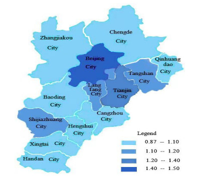
Utilizing statistical information from the Seventh National Population Census, statistical yearbook and sampling dynamic survey data, this study examines the distribution characteristics of the floating population in Beijing, Tianjin and Hebei Region as well as the growth trend of the floating population in each region. It also makes assessments using floating population concentration and The Moran Index Computing Methods. According to the study, the spatial distribution of the floating population has a clear clustering pattern in Beijing, Tianjin and Hebei region. Beijing, Tianjin and Hebei region's mobile population growth patterns differ substantially, and the region's inflow population is mostly made up of migrant inhabitants of domestic provinces and inflow of people from nearby regions. Most of the mobile population resides in Beijing and Tianjin, whereas the outflow of people originates in Hebei province. The diffusion impact and the spatial features of the floating population in the Beijing, Tianjin and Hebei area have a constant, positive association, according to the timeline between 2014 and 2020.

| [1] | H. S. Shryock, J. S. Siegel, The Methods and Materials of Demography, Academic Press, Salt Lake City, 1976. |
| [2] | C. Duan, The "mobile population" in China, Northwest Popul., 1 (1999), 2–5. |
| [3] | Q. Zhang, On the concept of population migration and mobile population, Popul. Res., 3 (1988), 17–18. |
| [4] | J. Li, A New Edition of Population Theory, China Population Press, Beijing, 2001. |
| [5] | C. Zhang, Z. Wang, Study on the rational distribution of population in China: spatial distribution of population and coordinated regional development, China Social Science Press, Beijing, 2015. |
| [6] |
E. G. Ravenstein, The laws of migration, J. Stat. Soc. London, 48 (1885), 167–235. https://doi.org/10.2307/2979181 doi: 10.2307/2979181

|
| [7] | R. Heberle, The causes of rural-urban migration a survey of German theories, Am. J. Sociol., 43 (1938), 932–950. |
| [8] | D. J. Bogue, Principles of Demography, Johnson Wiley and Sons, New York, 1969. |
| [9] |
E. S. Lee, A theory of migration, Demography, 3 (1966), 47–57. https://doi.org/10.2307/2060063 doi: 10.2307/2060063
|
| [10] |
W. A. Lewis, Economic development with unlimited supplies of labor, Manchester Sch., 22 (1954), 139–191. https://doi.org/10.1111/j.1467-9957.1954.tb00021.x doi: 10.1111/j.1467-9957.1954.tb00021.x
|
| [11] |
Z. Wang, Z. Jiang, D. Zheng, L. Wang, Study on the evolution of population spatial structure and optimization path of Beijing-Tianjin-Hebei urban groups, Northwest Popul. J., 37 (2016), 31–39. https://doi.org/10.15884/j.cnki.issn.1007-0672.2016.05.005 doi: 10.15884/j.cnki.issn.1007-0672.2016.05.005
|
| [12] | L. Xiao, X. Li, G. Zhang, R. Wang, Empirical analysis of social stratification of the resident population in Xiamen and policy recommendations, Prog. Geogr., 31 (2012), 183–190. |
| [13] | D. Huang, C. Lv, Characteristics of the evolution of the spatial pattern of Beijing's population-an analysis based on the 2000 and 2010 census data, Sci. Technol. Ind., 17 (2017), 107–114. |
| [14] |
R. M. Solow, Technical change and the aggregate production function, Rev. Econ. Stat., 39 (1957), 312–320. https://doi.org/10.2307/1926047 doi: 10.2307/1926047
|
| [15] | P. M. Romer, Increasing returns and new developments in the theory of growth, (1989), Available from: https://www.nber.org/papers/w3098 |
| [16] |
R. E. Lucas, On the mechanics of economic development, J. Monetary Econ., 22 (1988), 3–42. https://doi.org/10.1016/0304-3932(88)90168-7 doi: 10.1016/0304-3932(88)90168-7
|
| [17] | G. M. Grossman, E. Helpman, Innovation and Growth in the Global Economy, MIT press, Cambridge, 1993. |
| [18] |
D. T. Coe, E. Helpman, International R & D spillovers, Eur. Econ. Rev., 39 (1995), 859–887. https://doi.org/10.1016/0014-2921(94)00100-E doi: 10.1016/0014-2921(94)00100-E
|
| [19] |
A. A. Young, Increasing returns and economic progress, Econ. J., 38 (1928), 527–542. https://doi.org/10.2307/2224097 doi: 10.2307/2224097
|
| [20] | D. Zheng, Market size, division of labor, and endogenous growth models-and a discussion of whether endogenous growth theory misunderstands Young?, World Econ. Pap., (2015), 76–90. |
Figures(1) / Tables(5)

Lingling Wei, Haiyi Liu, Lifeng Wu. Spatial distribution of floating population in Beijing, Tianjin and Hebei Region and its correlations with synergistic development[J]. Mathematical Biosciences and Engineering, 2023, 20(3): 5949-5965. doi: 10.3934/mbe.2023257


 DownLoad: