3D human pose detection using nano sensor and multi-agent deep reinforcement learning

Yangjie Sun; Xiaoxi Che; Nan Zhang; Yangjie Sun; Xiaoxi Che; Nan Zhang

doi:10.3934/mbe.2023230

Mathematical Biosciences and Engineering

2023, Volume 20, Issue 3: 4970-4987. doi: 10.3934/mbe.2023230

Previous Article Next Article

Research article

3D human pose detection using nano sensor and multi-agent deep reinforcement learning

Physical Education Department, Beijing University of Technology, Beijing 100124, China

Received: 29 October 2022 Revised: 16 December 2022 Accepted: 19 December 2022 Published: 05 January 2023

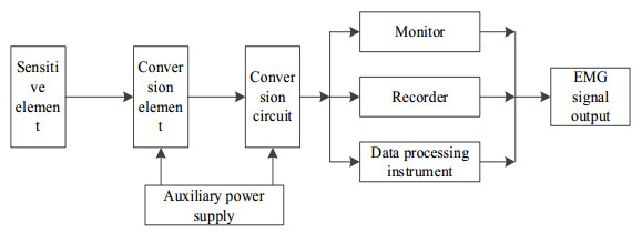
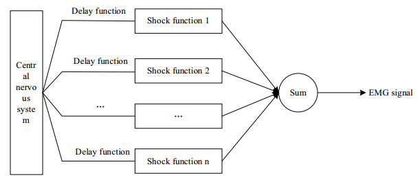
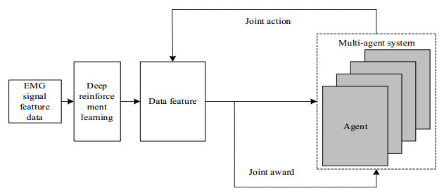
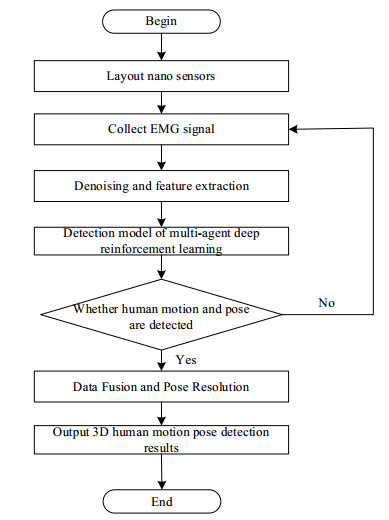
Due to the complexity of three-dimensional (3D) human pose, it is difficult for ordinary sensors to capture subtle changes in pose, resulting in a decrease in the accuracy of 3D human pose detection. A novel 3D human motion pose detection method is designed by combining Nano sensors and multi-agent deep reinforcement learning technology. First, Nano sensors are placed in key parts of the human to collect human electromyogram (EMG) signals. Second, after de-noising the EMG signal by blind source separation technology, the time-domain and frequency-domain features of the surface EMG signal are extracted. Finally, in the multi-agent environment, the deep reinforcement learning network is introduced to build the multi-agent deep reinforcement learning pose detection model, and the 3D local pose of the human is output according to the features of the EMG signal. The fusion and pose calculation of the multi-sensor pose detection results are performed to obtain the 3D human pose detection results. The results show that the proposed method has high accuracy for detecting various human poses, and the accuracy, precision, recall and specificity of 3D human pose detection results are 0.97, 0.98, 0.95 and 0.98, respectively. Compared with other methods, the detection results in this paper are more accurate, and can be widely used in medicine, film, sports and other fields.
- pose detection,
- EMG signal,
- feature extraction,
- nano sensor,
- multi-agent deep reinforcement learning,
- pose solution
Citation: Yangjie Sun, Xiaoxi Che, Nan Zhang. 3D human pose detection using nano sensor and multi-agent deep reinforcement learning[J]. Mathematical Biosciences and Engineering, 2023, 20(3): 4970-4987. doi: 10.3934/mbe.2023230

Related Papers:

Abstract

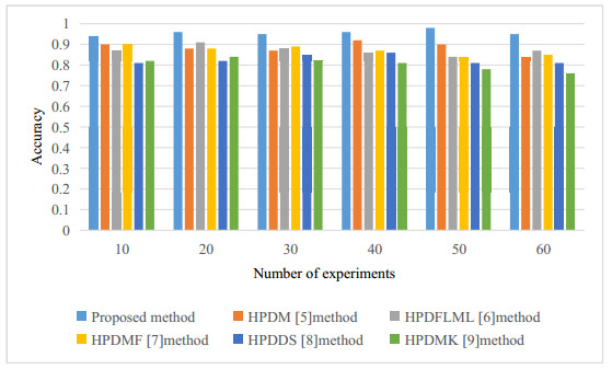
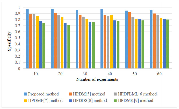
Due to the complexity of three-dimensional (3D) human pose, it is difficult for ordinary sensors to capture subtle changes in pose, resulting in a decrease in the accuracy of 3D human pose detection. A novel 3D human motion pose detection method is designed by combining Nano sensors and multi-agent deep reinforcement learning technology. First, Nano sensors are placed in key parts of the human to collect human electromyogram (EMG) signals. Second, after de-noising the EMG signal by blind source separation technology, the time-domain and frequency-domain features of the surface EMG signal are extracted. Finally, in the multi-agent environment, the deep reinforcement learning network is introduced to build the multi-agent deep reinforcement learning pose detection model, and the 3D local pose of the human is output according to the features of the EMG signal. The fusion and pose calculation of the multi-sensor pose detection results are performed to obtain the 3D human pose detection results. The results show that the proposed method has high accuracy for detecting various human poses, and the accuracy, precision, recall and specificity of 3D human pose detection results are 0.97, 0.98, 0.95 and 0.98, respectively. Compared with other methods, the detection results in this paper are more accurate, and can be widely used in medicine, film, sports and other fields.

References

[1]	L. Chen, S. Li, Human Motion target posture detection algorithm using semi-supervised learning in Internet of Things, IEEE Access, 9 (2021), 90529–90538. https://doi.org/10.1109/ACCESS.2021.3091430 doi: 10.1109/ACCESS.2021.3091430
[2]	M. Iwamoto, D. Kato, Efficient actor-critic reinforcement learning with embodiment of muscle tone for posture stabilization of the human arm, Neural Comput., 33 (2020), 1–28. https://doi.org/doi.org/10.1162/neco_a_01333 doi: 10.1162/neco_a_01333
[3]	A. Guzman-Pando, M. I. Chacon-Murguia, L. B. Chacon-Diaz, Human-like evaluation method for object motion detection algorithms, IET Computer Vision, 14 (2020), 674–682. https://doi.org/10.1049/iet-cvi.2019.0997 doi: 10.1049/iet-cvi.2019.0997
[4]	M. Wu, D. Du, Y. Li, W. Bai, W. Liu, Multi-cascade perceptual human posture recognition enhancement network, IEEE Access, 9 (2021), 64256–64266. https://doi.org/10.1109/ACCESS.2021.3074541 doi: 10.1109/ACCESS.2021.3074541
[5]	X. Song, L. Fan, Human posture recognition and estimation method based on 3D Multiview basketball sports dataset, Complexity, 25 (2021), 1–10. https://doi.org/10.1155/2021/6697697 doi: 10.1155/2021/6697697
[6]	W. Ren, O. Ma, H. Ji, X. Liu, Human posture recognition using a hybrid of fuzzy logic and machine learning approaches, IEEE Access, 8 (2020), 135628–135639. https://doi.org/10.1109/ACCESS.2020.3011697 doi: 10.1109/ACCESS.2020.3011697
[7]	W. Ding, B. Hu, H. Liu, X. M. Wang, X. S. Huang, Human posture recognition based on multiple features and rule learning, Int. J. Mach. Learn. Cyber, 11 (2020), 2529–2540. https://doi.org/10.1007/s13042-020-01138-y doi: 10.1007/s13042-020-01138-y
[8]	J. Wang, X. H. Liu, Human posture recognition method based on skeleton vector with depth sensor, IOP Conf. Ser. Mater. Sci. Eng., 806 (2020), 012035. https://doi.org/10.1088/1757-899X/806/1/012035 doi: 10.1088/1757-899X/806/1/012035
[9]	D. He, L. Li, A new Kinect-based posture recognition method in physical sports training based on urban data, Wireless Commun. Mobile Comput., 20 (2020), 1–9. https://doi.org/10.1155/2020/8817419 doi: 10.1155/2020/8817419
[10]	S. Liaqat, K. Dashtipour, K. Arshad, K. Assaleh, N. Ramzan, A hybrid posture detection framework: Integrating machine learning and deep neural networks, IEEE Sensors J., 21(2021), 9515–9522. https://doi.org/10.1109/JSEN.2021.3055898 doi: 10.1109/JSEN.2021.3055898
[11]	Z. Huang, J. Li, J. Huang, J. Ota, Y. Zhang, Motion planning for bandaging task with abnormal posture detection and avoidance, IEEE/ASME Transact. Mechatr., 25 (2020), 2364–2375. https://doi.org/10.1109/TMECH.2020.2973674 doi: 10.1109/TMECH.2020.2973674
[12]	H. Xia, X. Gao, Multi-scale mixed dense graph convolution network for skeleton-based action recognition, IEEE Access, 9 (2021), 36475–36484. https://doi.org/10.1109/ACCESS.2020.3049029 doi: 10.1109/ACCESS.2020.3049029
[13]	R. Xia, Y. Li, W. Luo, LAGA-Net: Local-and-global attention network for skeleton based action recognition, IEEE Transact. Multi., 24 (2022), 2648–2661. https://doi.org/10.1109/TMM.2021.3086758 doi: 10.1109/TMM.2021.3086758
[14]	Y. Kong, Y. Wang, A. Li, Spatiotemporal saliency representation learning for video action recognition, IEEE Transact. Multi., 24 (2022), 1515–1528. https://doi.org/10.1109/TMM.2021.3066775 doi: 10.1109/TMM.2021.3066775
[15]	M. Perez, J. Liu, A. C. Kot, Interaction relational network for mutual action recognition, IEEE Transact. Multi., 24 (2022), 366–376. https://doi.org/10.1109/TMM.2021.3050642 doi: 10.1109/TMM.2021.3050642
[16]	J. Xie, Q. G. Miao, R.Y Liu, W. T. Xin, L. Tang, S. Zhong, et al., Attention adjacency matrix based graph convolutional networks for skeleton-based action recognition, Neurocomputing, 440 (2021), 230–239. https://doi.org/10.1016/j.neucom.2021.02.001 doi: 10.1016/j.neucom.2021.02.001
[17]	D. Ludl, T. Gulde, C. Curio, Enhancing data-driven algorithms for human pose estimation and action recognition through simulation, IEEE Transact. Intell. Transport. Syst., 21 (2020), 3990–3999. https://doi.org/10.1109/TITS.2020.2988504 doi: 10.1109/TITS.2020.2988504
[18]	X. Ma, X. Li, Dynamic gesture contour feature extraction method using residual network transfer learning, Wireless Commun. Mobile Comput, 2021 (2021). https://doi.org/10.1155/2021/1503325 doi: 10.1155/2021/1503325
[19]	T. Ahmad, L. Jin, L. Lin, G. Z. Tang, Skeleton-based action recognition using sparse spatio-temporal GCN with edge effective resistance, Neurocomputing, 423 (2021), 389–398. https://doi.org/10.1016/j.neucom.2020.10.096 doi: 10.1016/j.neucom.2020.10.096
[20]	D. K. Vishwakarma, A two-fold transformation model for human action recognition using decisive pose, Cognit. Syst. Res., 61 (2020), 1–13. https://doi.org/10.1016/j.cogsys.2019.12.004 doi: 10.1016/j.cogsys.2019.12.004
[21]	Y. Lin, W. Chi, W. Sun, S. Liu, D. Fan, Human action recognition algorithm based on improved resnet and skeletal keypoints in single image, Math. Problems Eng., 12(2020), 1–12. https://doi.org/10.1155/2020/6954174 doi: 10.1155/2020/6954174

Reader Comments

Your name:*

Email:*
© 2023 the Author(s), licensee AIMS Press. This is an open access article distributed under the terms of the Creative Commons Attribution License (http://creativecommons.org/licenses/by/4.0)