DeepDN_iGlu: prediction of lysine glutarylation sites based on attention residual learning method and DenseNet

Jianhua Jia; Mingwei Sun; Genqiang Wu; Wangren Qiu; Jianhua Jia; Mingwei Sun; Genqiang Wu; Wangren Qiu

doi:10.3934/mbe.2023132

Mathematical Biosciences and Engineering

2023, Volume 20, Issue 2: 2815-2830. doi: 10.3934/mbe.2023132

Previous Article Next Article

Research article

DeepDN_iGlu: prediction of lysine glutarylation sites based on attention residual learning method and DenseNet

School of Information Engineering, Jingdezhen Ceramic University, Jingdezhen 333403, China

Academic Editor: Geng Dong

Received: 15 October 2022 Revised: 14 November 2022 Accepted: 17 November 2022 Published: 01 December 2022

As a key issue in orchestrating various biological processes and functions, protein post-translational modification (PTM) occurs widely in the mechanism of protein's function of animals and plants. Glutarylation is a type of protein-translational modification that occurs at active ε-amino groups of specific lysine residues in proteins, which is associated with various human diseases, including diabetes, cancer, and glutaric aciduria type I. Therefore, the issue of prediction for glutarylation sites is particularly important. This study developed a brand-new deep learning-based prediction model for glutarylation sites named DeepDN_iGlu via adopting attention residual learning method and DenseNet. The focal loss function is utilized in this study in place of the traditional cross-entropy loss function to address the issue of a substantial imbalance in the number of positive and negative samples. It can be noted that DeepDN_iGlu based on the deep learning model offers a greater potential for the glutarylation site prediction after employing the straightforward one hot encoding method, with Sensitivity (Sn), Specificity (Sp), Accuracy (ACC), Mathews Correlation Coefficient (MCC), and Area Under Curve (AUC) of 89.29%, 61.97%, 65.15%, 0.33 and 0.80 accordingly on the independent test set. To the best of the authors' knowledge, this is the first time that DenseNet has been used for the prediction of glutarylation sites. DeepDN_iGlu has been deployed as a web server (https://bioinfo.wugenqiang.top/~smw/DeepDN_iGlu/) that is available to make glutarylation site prediction data more accessible.
- post-translational modification,
- glutarylation site prediction,
- DenseNet,
- attention residual learning,
- focal loss function
Citation: Jianhua Jia, Mingwei Sun, Genqiang Wu, Wangren Qiu. DeepDN_iGlu: prediction of lysine glutarylation sites based on attention residual learning method and DenseNet[J]. Mathematical Biosciences and Engineering, 2023, 20(2): 2815-2830. doi: 10.3934/mbe.2023132

Related Papers:

Abstract

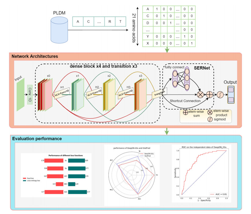
As a key issue in orchestrating various biological processes and functions, protein post-translational modification (PTM) occurs widely in the mechanism of protein's function of animals and plants. Glutarylation is a type of protein-translational modification that occurs at active ε-amino groups of specific lysine residues in proteins, which is associated with various human diseases, including diabetes, cancer, and glutaric aciduria type I. Therefore, the issue of prediction for glutarylation sites is particularly important. This study developed a brand-new deep learning-based prediction model for glutarylation sites named DeepDN_iGlu via adopting attention residual learning method and DenseNet. The focal loss function is utilized in this study in place of the traditional cross-entropy loss function to address the issue of a substantial imbalance in the number of positive and negative samples. It can be noted that DeepDN_iGlu based on the deep learning model offers a greater potential for the glutarylation site prediction after employing the straightforward one hot encoding method, with Sensitivity (Sn), Specificity (Sp), Accuracy (ACC), Mathews Correlation Coefficient (MCC), and Area Under Curve (AUC) of 89.29%, 61.97%, 65.15%, 0.33 and 0.80 accordingly on the independent test set. To the best of the authors' knowledge, this is the first time that DenseNet has been used for the prediction of glutarylation sites. DeepDN_iGlu has been deployed as a web server (https://bioinfo.wugenqiang.top/~smw/DeepDN_iGlu/) that is available to make glutarylation site prediction data more accessible.

References

[1]	E. Furuya, K. Uyeda, Regulation of phosphofructokinase by a new mechanism. An activation factor binding to phosphorylated enzyme, J. Biol. Chem., 255 (1980), 11656–11659. https://doi.org/10.1016/s0021-9258(19)70181-1 doi: 10.1016/s0021-9258(19)70181-1
[2]	C. Lu, C. B. Thompson, Metabolic regulation of epigenetics, Cell Metab., 16 (2012), 9–17. https://doi.org/10.1016/j.cmet.2012.06.001 doi: 10.1016/j.cmet.2012.06.001
[3]	M. Tan, C. Peng, K. A. Anderson, P. Chhoy, Z. Xie, L. Dai, et al., Lysine glutarylation is a protein posttranslational modification regulated by SIRT5, Cell Metab., 19 (2014), 605–617. https://doi.org/10.1016/j.cmet.2014.03.014 doi: 10.1016/j.cmet.2014.03.014
[4]	S. Ahmed, A. Rahman, M. Hasan, A. Mehedi, S. Ahmad, S. M. Shovan, Computational identification of multiple lysine PTM sites by analyzing the instance hardness and feature importance, Sci. Rep., 11 (2021), 18882. https://doi.org/10.1038/s41598-021-98458-y doi: 10.1038/s41598-021-98458-y
[5]	G. S. McDowell, A. Philpott, New insights into the role of ubiquitylation of proteins, Int. Rev. Cell Mol. Biol., 325 (2016), 35–88. https://doi.org/10.1016/bs.ircmb.2016.02.002 doi: 10.1016/bs.ircmb.2016.02.002
[6]	L. D. Vu, K. Gevaert, I. De Smet, Protein language: post-translational modifications talking to each other, Trends Plant Sci., 23 (2018), 1068–1080. https://doi.org/10.1016/j.tplants.2018.09.004 doi: 10.1016/j.tplants.2018.09.004
[7]	R. S. P. Rao, N. Zhang, D. Xu, I. M. Moller, CarbonylDB: a curated data-resource of protein carbonylation sites, Bioinformatics, 34 (2018), 2518–2520. https://doi.org/10.1093/bioinformatics/bty123 doi: 10.1093/bioinformatics/bty123
[8]	M. Wang, X. Cui, B. Yu, C. Chen, Q. Ma, H. Zhou, SulSite-GTB: identification of protein S-sulfenylation sites by fusing multiple feature information and gradient tree boosting, Neural Comput. Appl., 32 (2020), 13843–13862. https://doi.org/10.1007/s00521-020-04792-z doi: 10.1007/s00521-020-04792-z
[9]	X. Liu, L. Wang, J. Li, J. Hu, X. Zhang, Mal-Prec: computational prediction of protein Malonylation sites via machine learning based feature integration, BMC Genomics, 21 (2020), 812. https://doi.org/10.1186/s12864-020-07166-w doi: 10.1186/s12864-020-07166-w
[10]	K. Y. Huang, F. Y. Hung, H. J. Kao, H. H. Lau, S. L. Weng, iDPGK: characterization and identification of lysine phosphoglycerylation sites based on sequence-based features, BMC Bioinf., 21 (2020), 568. https://doi.org/10.1186/s12859-020-03916-5 doi: 10.1186/s12859-020-03916-5
[11]	S. Ahmed, M. Kabir, M. Arif, Z. U. Khan, D. J. Yu, DeepPPSite: a deep learning-based model for analysis and prediction of phosphorylation sites using efficient sequence information, Anal. Biochem., 612 (2021), 113955. https://doi.org/10.1016/j.ab.2020.113955 doi: 10.1016/j.ab.2020.113955
[12]	N. Thapa, M. Chaudhari, S. McManus, K. Roy, R. H. Newman, H. Saigo, et al., DeepSuccinylSite: a deep learning based approach for protein succinylation site prediction, BMC Bioinf., 21 (2020), 63. https://doi.org/10.1186/s12859-020-3342-z doi: 10.1186/s12859-020-3342-z
[13]	Z. Ju, J. J. He, Prediction of lysine glutarylation sites by maximum relevance minimum redundancy feature selection, Anal. Biochem., 550 (2018), 1–7. https://doi.org/10.1016/j.ab.2018.04.005 doi: 10.1016/j.ab.2018.04.005
[14]	Y. Xu, Y. Yang, J. Ding, C. Li, iGlu-Lys: A Predictor for lysine glutarylation through amino acid pair order features, IEEE Trans. Nanobiosci., 17 (2018), 394–401. https://doi.org/10.1109/TNB.2018.2848673 doi: 10.1109/TNB.2018.2848673
[15]	K. Y. Huang, H. J. Kao, J. B. K. Hsu, S. L. Weng, T. Y. Lee, Characterization and identification of lysine glutarylation based on intrinsic interdependence between positions in the substrate sites, BMC Bioinf., 19 (2019), 13–25. https://doi.org/10.1186/s12859-018-2394-9 doi: 10.1186/s12859-018-2394-9
[16]	H. J. Al-Barakati, H. Saigo, R. H. Newman, D. B. KC, RF-GlutarySite: a random forest based predictor for glutarylation sites, Mol. Omics, 15 (2019), 189–204. https://doi.org/10.1039/c9mo00028c doi: 10.1039/c9mo00028c
[17]	M. E. Arafat, M. W. Ahmad, S. M. Shovan, A. Dehzangi, S. R. Dipta, M. A. M. Hasan, et al., Accurately predicting glutarylation sites using sequential Bi-Peptide-Based evolutionary features, Genes, 11 (2020), 1023. https://doi.org/10.3390/genes11091023 doi: 10.3390/genes11091023
[18]	L. Dou, X. Li, L. Zhang, H. Xiang, L. Xu, iGlu_AdaBoost: identification of lysine glutarylation using the adaboost classifier, J. Proteome Res., 20 (2020), 191–201. https://doi.org/10.1021/acs.jproteome.0c00314 doi: 10.1021/acs.jproteome.0c00314
[19]	J. Jia, Z. Liu, X. Xian, B. Liu, K. C. Chou, pSuc-Lys: Predict lysine succinylation sites in proteins with PseAAC and ensemble random forest approach, J. Theor. Biol., 394 (2016), 223–230. https://doi.org/10.1016/j.jtbi.2016.01.020 doi: 10.1016/j.jtbi.2016.01.020
[20]	P. Kelchtermans, W. Bittremieux, K. De Grave, S. Degroeve, J. Ramon, K. Laukens, et al., Machine learning applications in proteomics research: how the past can boost the future, Proteomics, 14 (2014), 353–366. https://doi.org/10.1002/pmic.201300289 doi: 10.1002/pmic.201300289
[21]	L. Dou, F. Yang, L. Xu, Q. Zou, A comprehensive review of the imbalance classification of protein post-translational modifications, Briefings Bioinf., 22 (2021), bbab089. https://doi.org/10.1093/bib/bbab089 doi: 10.1093/bib/bbab089
[22]	Z. Ju, S. Y. Wang, Computational identification of lysine glutarylation sites using positive-unlabeled learning, Curr. Genomics, 21 (2020), 204–211. https://doi.org/10.2174/1389202921666200511072327 doi: 10.2174/1389202921666200511072327
[23]	B. Wen, W. F. Zeng, Y. Liao, Z. Shi, S. R. Savage, W. Jiang, et al., Deep learning in proteomics, Proteomics, 20 (2020), 1900335. https://doi.org/10.1002/pmic.201900335 doi: 10.1002/pmic.201900335
[24]	S. C. Pakhrin, S. Pokharel, H. Saigo, D. B. Kc, Deep learning-based advances in protein posttranslational modification site and protein cleavage prediction, in Computational Methods for Predicting Post-Translational Modification Sites, Humana Press, (2022), 285–322. https://doi.org/10.1007/978-1-0716-2317-6_15
[25]	S. Naseer, R. F. Ali, Y. D. Khan, P. D. D. Dominic, iGluK-Deep: computational identification of lysine glutarylation sites using deep neural networks with general pseudo amino acid compositions, J. Biomol. Struct. Dyn., 2021 (2021), 1–14. https://doi.org/10.1080/07391102.2021.1962738 doi: 10.1080/07391102.2021.1962738
[26]	C. M. Liu, V. D. Ta, N. Q. K. Le, D. A. Tadesse, C. Shi, Deep neural network framework based on word embedding for protein glutarylation sites prediction, Life, 12 (2022), 1213. https://doi.org/10.3390/life12081213 doi: 10.3390/life12081213
[27]	H. Xu, J. Zhou, S. Lin, W. Deng, Y. Zhang, Y. Xue, PLMD: an updated data resource of protein lysine modifications, J. Genet. Genomics, 44 (2017), 243–250. https://doi.org/10.1016/j.jgg.2017.03.007 doi: 10.1016/j.jgg.2017.03.007
[28]	W. Li, A. Godzik, Cd-hit: a fast program for clustering and comparing large sets of protein or nucleotide sequences, Bioinformatics, 22 (2006), 1658–1659. https://doi.org/10.1093/bioinformatics/btl158 doi: 10.1093/bioinformatics/btl158
[29]	Y. Huang, B. Niu, Y. Gao, L. Fu, W. Li, CD-HIT Suite: a web server for clustering and comparing biological sequences, Bioinformatics, 26 (2010), 680–682. https://doi.org/10.1093/bioinformatics/btq003 doi: 10.1093/bioinformatics/btq003
[30]	K. C. Chou, Prediction of signal peptides using scaled window, Peptides, 22 (2001), 1973–1979. https://doi.org/10.1016/S0196-9781(01)00540-X doi: 10.1016/S0196-9781(01)00540-X
[31]	H. Wang, H. Zhao, Z. Yan, J. Zhao, J. Han, MDCAN-Lys: a model for predicting succinylation sites based on multilane dense convolutional attention network, Biomolecules, 11 (2021), 872. https://doi.org/10.3390/biom11060872 doi: 10.3390/biom11060872
[32]	H. Wang, Z. Yan, D. Liu, H. Zhao, J. Zhao, MDC-Kace: A model for predicting lysine acetylation sites based on modular densely connected convolutional networks, IEEE Access, 8 (2020), 214469–214480. https://doi.org/10.1109/access.2020.3041044 doi: 10.1109/access.2020.3041044
[33]	G. Huang, Z. Liu, L. Van Der Maaten, K. Q. Weinberger, Densely connected convolutional networks, in 2017 IEEE Conference on Computer Vision and Pattern Recognition (CVPR), Honolulu, USA, (2017), 2261–2269. http://doi.org/10.1109/CVPR.2017.243
[34]	T. Y. Lin, P. Goyal, R. Girshick, K. He, P. Dollár, Focal loss for dense object detection, in Proceedings of the IEEE International Conference on Computer Vision, Venice, Italy, (2017), 2999–3007. https://doi.org/10.1109/ICCV.2017.324
[35]	M. Sokolova, G. Lapalme, A systematic analysis of performance measures for classification tasks, Inf. Process. Manage., 45 (2009), 427–437. https://doi.org/10.1016/j.ipm.2009.03.002 doi: 10.1016/j.ipm.2009.03.002
[36]	S. Boughorbel, F. Jarray, M. El-Anbari, Optimal classifier for imbalanced data using Matthews Correlation Coefficient metric, PLoS One, 12 (2017), e0177678. https://doi.org/10.1371/journal.pone.0177678 doi: 10.1371/journal.pone.0177678
[37]	T. Fawcett, An introduction to ROC analysis, Pattern Recognit. Lett., 27 (2006), 861–874. https://doi.org/10.1016/j.patrec.2005.10.010 doi: 10.1016/j.patrec.2005.10.010

Reader Comments

Your name:*

Email:*
© 2023 the Author(s), licensee AIMS Press. This is an open access article distributed under the terms of the Creative Commons Attribution License (http://creativecommons.org/licenses/by/4.0)