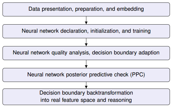
A probabilistic neural network has been implemented to predict the malignancy of breast cancer cells, based on a data set, the features of which are used for the formulation and training of a model for a binary classification problem. The focus is placed on considerations when building the model, in order to achieve not only accuracy but also a safe quantification of the expected uncertainty of the calculated network parameters and the medical prognosis. The source code is included to make the results reproducible, also in accordance with the latest trending in machine learning research, named Papers with Code. The various steps taken for the code development are introduced in detail but also the results are visually displayed and critically analyzed also in the sense of explainable artificial intelligence. In statistical-classification problems, the decision boundary is the region of the problem space in which the classification label of the classifier is ambiguous. Problem aspects and model parameters which influence the decision boundary are a special aspect of practical investigation considered in this work. Classification results issued by technically transparent machine learning software can inspire more confidence, as regards their trustworthiness which is very important, especially in the case of medical prognosis. Furthermore, transparency allows the user to adapt models and learning processes to the specific needs of a problem and has a boosting influence on the development of new methods in relevant machine learning fields (transfer learning).
Citation: Anastasia-Maria Leventi-Peetz, Kai Weber. Probabilistic machine learning for breast cancer classification[J]. Mathematical Biosciences and Engineering, 2023, 20(1): 624-655. doi: 10.3934/mbe.2023029
A probabilistic neural network has been implemented to predict the malignancy of breast cancer cells, based on a data set, the features of which are used for the formulation and training of a model for a binary classification problem. The focus is placed on considerations when building the model, in order to achieve not only accuracy but also a safe quantification of the expected uncertainty of the calculated network parameters and the medical prognosis. The source code is included to make the results reproducible, also in accordance with the latest trending in machine learning research, named Papers with Code. The various steps taken for the code development are introduced in detail but also the results are visually displayed and critically analyzed also in the sense of explainable artificial intelligence. In statistical-classification problems, the decision boundary is the region of the problem space in which the classification label of the classifier is ambiguous. Problem aspects and model parameters which influence the decision boundary are a special aspect of practical investigation considered in this work. Classification results issued by technically transparent machine learning software can inspire more confidence, as regards their trustworthiness which is very important, especially in the case of medical prognosis. Furthermore, transparency allows the user to adapt models and learning processes to the specific needs of a problem and has a boosting influence on the development of new methods in relevant machine learning fields (transfer learning).

| [1] |
Q. Xia, Y. Cheng, J. Hu, J. Huang, Y. Yu, H. Xie, J. Wang, Differential diagnosis of breast cancer assisted by S-Detect artificial intelligence system, Math. Biosci. Eng., 18 (2021), 3680–3689. https://doi.org/10.3934/mbe.2021184 doi: 10.3934/mbe.2021184

|
| [2] |
X. Zhang, Z. Yu, Pathological analysis of hesperetin-derived small cell lung cancer by artificial intelligence technology under fiberoptic bronchoscopy, Math. Biosci. Eng., 18 (2021), 8538–8558. https://doi.org/10.3934/mbe.2021423 doi: 10.3934/mbe.2021423
|
| [3] |
S. Biswas, D. Sen, D. Bhatia, P. Phukan, M. Mukherjee, Chest X-Ray image and pathological data based artificial intelligence enabled dual diagnostic method for multi-stage classification of COVID-19 patients, AIMS Biophys., 8 (2021), 346–371. https://doi.org/10.3934/biophy.2021028 doi: 10.3934/biophy.2021028
|
| [4] |
T. Ayer, J. Chhatwal, O. Alagoz, C. E. Kahn, R. W. Woods, E. S. Burnside, Comparison of logistic regression and artificial neural network models in breast cancer risk estimation, Radiographics, 30 (2010), 13–21. https://doi.org/10.1148/rg.301095057 doi: 10.1148/rg.301095057
|
| [5] | T. van der Ploeg, M. Smits, D. W. Dippel, M. Hunink, E. W. Steyerberg, Prediction of intracranial findings on CT-scans by alternative modelling techniques, BMC Med. Res. Methodol., 11 (2011). https://doi.org/10.1186/1471-2288-11-143 |
| [6] |
L. V. Jospin, W. L. Buntine, F. Boussaïd, H. Laga, M. Bennamoun, Hands-On Bayesian neural networks – A tutorial for deep learning users, IEEE Comput. Intell. Mag., 17 (2022), 29–48. https://doi.org/10.1109/MCI.2022.3155327 doi: 10.1109/MCI.2022.3155327
|
| [7] |
A. A. Abdullah, M. M. Hassan, Y. T. Mustafa, A review on Bayesian deep learning in healthcare: Applications and challenges, IEEE Access, 10 (2022), 36538–36562. https://doi.org/10.1109/ACCESS.2022.3163384 doi: 10.1109/ACCESS.2022.3163384
|
| [8] |
E. Hüllermeier, W. Waegeman, Aleatoric and epistemic uncertainty in machine learning: An introduction to concepts and methods, Mach. Learn., 110 (2021), 457–506. https://doi.org/10.1007/s10994-021-05946-3 doi: 10.1007/s10994-021-05946-3
|
| [9] | G. Deodato, Uncertainty modeling in deep learning, Variational inference for Bayesian neural networks, 2019. Available from: http://webthesis.biblio.polito.it/id/eprint/10920. |
| [10] | H. Huang, Y. Wang, C. Rudin, E. P. Browne, Towards a comprehensive evaluation of dimension reduction methods for transcriptomic data visualization, Commun. Biol., 5 (2022). https://doi.org/10.1038/s42003-022-03628-x |
| [11] | L. McInnes, J. Healy, J. Melville, UMAP: Uniform manifold approximation and projection for dimension reduction, preprint, arXiv: 1802.03426. https://doi.org/10.48550/arXiv.1802.03426 |
| [12] |
A. Diaz-Papkovich, L. Anderson-Trocmé, S. Gravel, A review of UMAP in population genetics, J. Hum. Genet., 66 (2021), 85–91. https://doi.org/10.1038/s10038-020-00851-4 doi: 10.1038/s10038-020-00851-4
|
| [13] |
J. Salvatier, T. V. Wiecki, C. Fonnesbeck, Probabilistic programming in Python using PyMC3, PeerJ Comput. Sci., 2 (2016), e55. https://doi.org/10.7717/peerj-cs.55 doi: 10.7717/peerj-cs.55
|
| [14] |
A. Kucukelbir, D. Tran, R. Ranganath, A. Gelman, D. M. Blei, David M., Automatic differentiation variational inference, J. Mach. Learn. Res., 18 (2017), 1–45. https://doi.org/10.48550/arXiv.1603.00788 doi: 10.48550/arXiv.1603.00788
|
| [15] | M. Krasser, Variational inference in Bayesian neural networks. Available from: http://krasserm.github.io/2019/03/14/bayesian-neural-networks/. |
| [16] | L. van der Maaten, G. Hinton, Visualizing data using t-SNE, J. Mach. Learn. Res., 9 (2008), 2579–2605. |
| [17] | F. Pedregosa, G. Varoquaux, A. Gramfort, V. Michel, B. Thirion, O. Grisel, et al., Scikit-learn: Machine learning in Python, J. Mach. Learn. Res., 12 (2011), 2825–2830. |
| [18] | Heaton Research, The number of hidden layers. Available from: https://www.heatonresearch.com/2017/06/01/hidden-layers.html. |
| [19] | T. Wood, What is the Sigmoid Function?, 2020. Available from: https://deepai.org/machine-learning-glossary-and-terms/sigmoid-function. |
| [20] | A. K. Dhaka, A. Catalina, M. R. Andersen, M. Magnusson, J. H. Huggins, A. Vehtari, Robust, accurate stochastic optimization for variational inference, in Advances in Neural Information Processing Systems (eds. H. Larochelle et al.), Curran Associates, Inc., 33 (2020), 10961–10973. |
| [21] |
A. Gelman, B. Carpenter, Bayesian analysis of tests with unknown specificity and sensitivity, J. R. Stat. Soc. Ser. C, 69 (2020), 1269–1283. https://doi.org/10.1111/rssc.12435 doi: 10.1111/rssc.12435
|
| [22] | D. Lunn, C. Jackson, N. Best, A. Thomas, D. Spiegelhalter, The BUGS book: A practical introduction to Bayesian analysis, Chapman and Hall/CRC, Boca Raton, USA, 2012. |
| [23] | D. B. Rizzo, M. R. Blackburn, Harnessing expert knowledge: Defining Bayesian network model priors from expert knowledge only–prior elicitation for the vibration qualification problem IEEE Syst. J., 13 (2019), 1895–1905. https://doi.org/10.1109/JSYST.2019.2892942 |
| [24] | A. M. Stefan, D. Katsimpokis, Q. F. Gronau, E. J. Wagenmakers, Expert agreement in prior elicitation and its effects on Bayesian inference, Psychon. Bull. Rev., 2022. https://doi.org/10.3758/s13423-022-02074-4 |
| [25] | V. Fortuin, Priors in Bayesian deep learning: A review, Int. Stat. Rev., 2022. https://doi.org/10.1111/insr.12502 |
| [26] |
C. Esposito, G. A. Landrum, N. Schneider, N. Stiefl, S. Riniker, GHOST: Adjusting the decision threshold to handle imbalanced data in machine learning, J. Chem. Inf. Model., 61 (2021), 2623–2640. https://doi.org/10.1021/acs.jcim.1c00160 doi: 10.1021/acs.jcim.1c00160
|
| [27] |
Q. Kim, J.-H. Ko, S. Kim, N. Park, W. Jhe, Bayesian neural network with pretrained protein embedding enhances prediction accuracy of drug-protein interaction, Bioinformatics, 37 (2021), 3428–3435. https://doi.org/10.1093/bioinformatics/btab346 doi: 10.1093/bioinformatics/btab346
|
| [28] |
S. Budd, E. C. Robinson, B. Kainz, A Survey on active learning and human-in-the-Loop deep learning for medical image analysis, Med. Image Anal., 71 (2021), 102062. https://doi.org/10.1016/j.media.2021.102062 doi: 10.1016/j.media.2021.102062
|
| [29] | V. S. Bisen, What is Human in the Loop Machine Learning: Why & How Used in AI?, 2020. Available from: https://medium.com/vsinghbisen/what-is-human-in-the-loop-machine-learning-why-how-used-in-ai-60c7b44eb2c0. |
| [30] | K. Bykov, M. M. C. Höhne, A. Creosteanu, K. R. Müller, F. Klauschen, S. Nakajima, et al., Explaining Bayesian neural networks, preprint, arXiv: 2108.10346. https://doi.org/10.48550/arXiv.2108.10346 |


Figures(17) / Tables(2)

Anastasia-Maria Leventi-Peetz, Kai Weber. Probabilistic machine learning for breast cancer classification[J]. Mathematical Biosciences and Engineering, 2023, 20(1): 624-655. doi: 10.3934/mbe.2023029


 DownLoad: