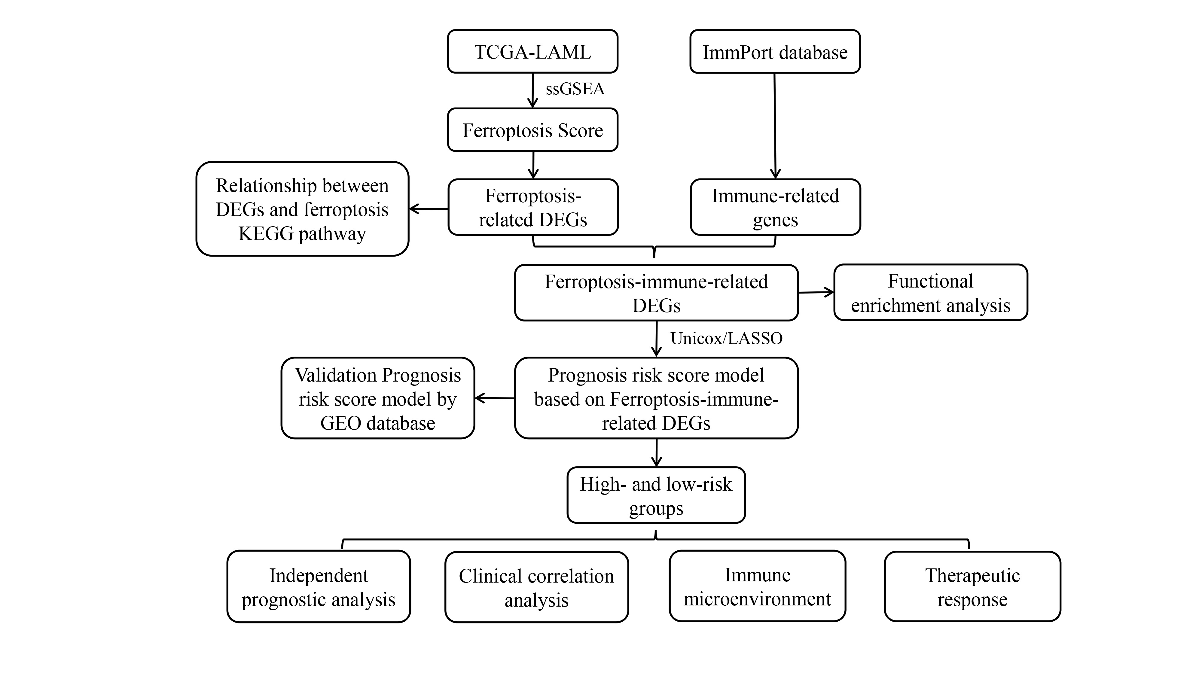
In acute myeloid leukemia (AML), the link between ferroptosis and the immune microenvironment has profound clinical significance. The objective of this study was to investigate the role of ferroptosis-immune related genes (FIRGs) in predicting the prognosis and therapeutic sensitivity in patients with AML. Using The Cancer Genome Atlas dataset, single sample gene set enrichment analysis was performed to calculate the ferroptosis score of AML samples. To search for FIRGs, differentially expressed genes between the high- and low-ferroptosis score groups were identified and then cross-screened with immune related genes. Univariate Cox and LASSO regression analyses were performed on the FIRGs to establish a prognostic risk score model with five signature FIRGs (BMP2, CCL3, EBI3, ELANE, and S100A6). The prognostic risk score model was then used to divide the patients into high- and low-risk groups. For external validation, two Gene Expression Omnibus cohorts were employed. Overall survival was poorer in the high-risk group than in the low-risk group. The novel risk score model was an independent prognostic factor for overall survival in patients with AML. Infiltrating immune cells were also linked to high-risk scores. Treatment targeting programmed cell death protein 1 may be more effective in high-risk patients. This FIRG-based prognostic risk model may aid in optimizing prognostic risk stratification and treatment of AML.
Citation: Xing Guo, Xiaogang Zhou. Risk stratification of acute myeloid leukemia: Assessment using a novel prediction model based on ferroptosis-immune related genes[J]. Mathematical Biosciences and Engineering, 2022, 19(12): 11821-11839. doi: 10.3934/mbe.2022551
In acute myeloid leukemia (AML), the link between ferroptosis and the immune microenvironment has profound clinical significance. The objective of this study was to investigate the role of ferroptosis-immune related genes (FIRGs) in predicting the prognosis and therapeutic sensitivity in patients with AML. Using The Cancer Genome Atlas dataset, single sample gene set enrichment analysis was performed to calculate the ferroptosis score of AML samples. To search for FIRGs, differentially expressed genes between the high- and low-ferroptosis score groups were identified and then cross-screened with immune related genes. Univariate Cox and LASSO regression analyses were performed on the FIRGs to establish a prognostic risk score model with five signature FIRGs (BMP2, CCL3, EBI3, ELANE, and S100A6). The prognostic risk score model was then used to divide the patients into high- and low-risk groups. For external validation, two Gene Expression Omnibus cohorts were employed. Overall survival was poorer in the high-risk group than in the low-risk group. The novel risk score model was an independent prognostic factor for overall survival in patients with AML. Infiltrating immune cells were also linked to high-risk scores. Treatment targeting programmed cell death protein 1 may be more effective in high-risk patients. This FIRG-based prognostic risk model may aid in optimizing prognostic risk stratification and treatment of AML.

| [1] |
K. Sasaki, F. Ravandi, T. M. Kadia, C. D. DiNardo, N. J. Short, G. Borthakur, et al., De novo acute myeloid leukemia: A population-based study of outcome in the United States based on the Surveillance, Epidemiology, and End Results (SEER) database, 1980 to 2017, Cancer, 127 (2021), 2049–2061. https://doi.org/10.1002/cncr.33458 doi: 10.1002/cncr.33458

|
| [2] |
C. Ganzel, Z. Sun, L. D. Cripe, H. F. Fernandez, D. Douer, J. M. Rowe, et al., Very poor long-term survival in past and more recent studies for relapsed AML patients: The ECOG-ACRIN experience, Am. J. Hematol., 93 (2018), 1074–1081. https://doi.org/10.1002/ajh.25162 doi: 10.1002/ajh.25162
|
| [3] |
S. J. Dixon, K. M. Lemberg, M. R. Lamprecht, R. Skouta, E. M. Zaitsev, C. E. Gleason, et al., Ferroptosis: an iron-dependent form of nonapoptotic cell death, Cell, 149 (2012), 1060–1072. https://doi.org/10.1016/j.cell.2012.03.042 doi: 10.1016/j.cell.2012.03.042
|
| [4] |
B. Hassannia, P. Vandenabeele, T. V. Berghe, Targeting ferroptosis to iron out cancer, Cancer Cell, 35 (2019), 830–849. https://doi.org/10.1016/j.ccell.2019.04.002 doi: 10.1016/j.ccell.2019.04.002
|
| [5] |
C. Liang, X. Zhang, M. Yang, X. Dong, Recent progress in ferroptosis inducers for cancer therapy, Adv. Mater., 31 (2019), e1904197. https://doi.org/10.1002/adma.201904197 doi: 10.1002/adma.201904197
|
| [6] |
F. Zhang, H. Liu, Identification of ferroptosis-associated genes exhibiting altered expression in pulmonary arterial hypertension, Math. Biosci. Eng., 18 (2021), 7619–7630. https://doi.org/10.3934/mbe.2021377 doi: 10.3934/mbe.2021377
|
| [7] |
R. Birsen, C. Larrue, J. Decroocq, N. Johnson, N. Guiraud, M. Gotanegre, et al., APR-246 induces early cell death by ferroptosis in acute myeloid leukemia, Haematologica, 107 (2022), 403–416. https://doi.org/10.3324/haematol.2020.259531 doi: 10.3324/haematol.2020.259531
|
| [8] |
D. S. Liu, C. P. Duong, S. Haupt, K. G. Montgomery, C. M. House, W. J. Azar, et al., Inhibiting the system xC(-)/glutathione axis selectively targets cancers with mutant-p53 accumulation, Nat. Commun., 8 (2017), 14844. https://doi.org/10.1038/ncomms14844 doi: 10.1038/ncomms14844
|
| [9] |
H. Liu, Emerging agents and regimens for AML, J. Hematol. Oncol., 14 (2021), 49. https://doi.org/10.1186/s13045-021-01062-w doi: 10.1186/s13045-021-01062-w
|
| [10] |
Q. Zheng, Y. Zhao, J. Guo, S. Zhao, C. Fei, C. Xiao, et al., Iron overload promotes mitochondrial fragmentation in mesenchymal stromal cells from myelodysplastic syndrome patients through activation of the AMPK/MFF/Drp1 pathway, Cell Death Dis., 9 (2018), 515. https://doi.org/10.1038/s41419-018-0552-7 doi: 10.1038/s41419-018-0552-7
|
| [11] |
H. Tanaka, J. L. Espinoza, R. Fujiwara, S. Rai, Y. Morita, T. Ashida, et al., Excessive reactive iron impairs hematopoiesis by affecting both immature hematopoietic cells and stromal cells, Cells, 8 (2019). https://doi.org/10.3390/cells8030226 doi: 10.3390/cells8030226
|
| [12] |
V. D. Turubanova, I. V. Balalaeva, T. A. Mishchenko, E. Catanzaro, R. Alzeibak, N. N. Peskova, et al., Immunogenic cell death induced by a new photodynamic therapy based on photosens and photodithazine, J. Immunother. Cancer, 7 (2019), 350. https://doi.org/10.1186/s40425-019-0826-3 doi: 10.1186/s40425-019-0826-3
|
| [13] |
W. Wang, M. Green, J. E. Choi, M. Gijon, P. D. Kennedy, J. K. Johnson, et al., CD8+ T cells regulate tumour ferroptosis during cancer immunotherapy, Nature, 569 (2019), 270–274. https://doi.org/10.1038/s41586-019-1170-y doi: 10.1038/s41586-019-1170-y
|
| [14] |
D. H. Kim, W. D. Kim, S. K. Kim, D. H. Moon, S. J. Lee, TGF-beta1-mediated repression of SLC7A11 drives vulnerability to GPX4 inhibition in hepatocellular carcinoma cells, Cell Death Dis., 11 (2020), 406. https://doi.org/10.1038/s41419-020-2618-6 doi: 10.1038/s41419-020-2618-6
|
| [15] |
M. Manzano, A. Patil, A. Waldrop, S. S. Dave, A. Behdad, E. Gottwein, Gene essentiality landscape and druggable oncogenic dependencies in herpesviral primary effusion lymphoma, Nat. Commun., 9 (2018), 3263. https://doi.org/10.1038/s41467-018-05506-9 doi: 10.1038/s41467-018-05506-9
|
| [16] |
Y. Teng, B. Wang, D. Shang, N. Yang, Identification and validation of an immune and ferroptosis-combined index for non-small cell lung cancer, Front. Genet., 12 (2021), 764869. https://doi.org/10.3389/fgene.2021.764869 doi: 10.3389/fgene.2021.764869
|
| [17] |
B. Tang, R. Yan, J. Zhu, S. Cheng, C. Kong, W. Chen, et al., Integrative analysis of the molecular mechanisms, immunological features and immunotherapy response of ferroptosis regulators across 33 cancer types, Int. J. Biol. Sci., 18 (2022), 180–198. https://doi.org/10.7150/ijbs.64654 doi: 10.7150/ijbs.64654
|
| [18] |
B. N. Ostendorf, J. Bilanovic, N. Adaku, K. N. Tafreshian, B. Tavora, R. D. Vaughan, et al., Common germline variants of the human APOE gene modulate melanoma progression and survival, Nat. Med., 26 (2020), 1048–1053. https://doi.org/10.1038/s41591-020-0879-3 doi: 10.1038/s41591-020-0879-3
|
| [19] |
N. Kim, H. K. Kim, K. Lee, Y. Hong, J. H. Cho, J. W. Choi, et al., Single-cell RNA sequencing demonstrates the molecular and cellular reprogramming of metastatic lung adenocarcinoma, Nat. Commun., 11 (2020), 2285. https://doi.org/10.1038/s41467-020-16164-1 doi: 10.1038/s41467-020-16164-1
|
| [20] |
M. E. Ritchie, B. Phipson, D. Wu, Y. Hu, C. W. Law, W. Shi, et al., limma powers differential expression analyses for RNA-sequencing and microarray studies, Nucleic Acids Res., 43 (2015), e47. https://doi.org/10.1093/nar/gkv007 doi: 10.1093/nar/gkv007
|
| [21] |
G. Yu, L. G. Wang, Y. Han, Q. Y. He, clusterProfiler: an R package for comparing biological themes among gene clusters, OMICS, 16 (2012), 284–287. https://doi.org/10.1089/omi.2011.0118 doi: 10.1089/omi.2011.0118
|
| [22] |
N. Simon, J. Friedman, T. Hastie, R. Tibshirani, Regularization paths for cox's proportional hazards model via coordinate descent, J. Stat. Softw., 39 (2011), 1–13. https://doi.org/10.18637/jss.v039.i05 doi: 10.18637/jss.v039.i05
|
| [23] |
R. Tibshirani, The lasso method for variable selection in the Cox model, Stat. Med., 16 (1997), 385–395. https://doi.org/10.1002/(sici)1097-0258(19970228)16:4<385::aid-sim380>3.0.co;2-3 doi: 10.1002/(sici)1097-0258(19970228)16:4<385::aid-sim380>3.0.co;2-3
|
| [24] |
S. Stanley, K. Vanarsa, S. Soliman, D. Habazi, C. Pedroza, G. Gidley, et al., Comprehensive aptamer-based screening identifies a spectrum of urinary biomarkers of lupus nephritis across ethnicities, Nat. Commun., 11 (2020), 2197. https://doi.org/10.1038/s41467-020-15986-3 doi: 10.1038/s41467-020-15986-3
|
| [25] |
Y. Wang, F. Hu, J. Y. Li, R. C. Nie, S. L. Chen, Y. Y. Cai, et al., Systematic construction and validation of a metabolic risk model for prognostic prediction in acute myelogenous leukemia, Front. Oncol., 10 (2020), 540. https://doi.org/10.3389/fonc.2020.00540 doi: 10.3389/fonc.2020.00540
|
| [26] |
S. Ullrich, R. Guigo, Dynamic changes in intron retention are tightly associated with regulation of splicing factors and proliferative activity during B-cell development, Nucleic Acids Res., 48 (2020), 1327–1340. https://doi.org/10.1093/nar/gkz1180 doi: 10.1093/nar/gkz1180
|
| [27] |
B. Bengsch, T. Ohtani, O. Khan, M. Setty, S. Manne, S. O'Brien, et al., Epigenomic-guided mass cytometry profiling reveals disease-specific features of exhausted CD8 T cells, Immunity, 48 (2018), 1029–1045. https://doi.org/10.1016/j.immuni.2018.04.026 doi: 10.1016/j.immuni.2018.04.026
|
| [28] |
X. Tekpli, T. Lien, A. H. Rossevold, D. Nebdal, E. Borgen, H. O. Ohnstad, et al., An independent poor-prognosis subtype of breast cancer defined by a distinct tumor immune microenvironment, Nat. Commun., 10 (2019), 5499. https://doi.org/10.1038/s41467-019-13329-5 doi: 10.1038/s41467-019-13329-5
|
| [29] |
Y. Song, S. Tian, P. Zhang, N. Zhang, Y. Shen, J. Deng, Construction and validation of a novel ferroptosis-related prognostic model for acute myeloid leukemia, Front. Genet., 12 (2021), 708699. https://doi.org/10.3389/fgene.2021.708699 doi: 10.3389/fgene.2021.708699
|
| [30] |
N. Jiang, X. Zhang, Q. Chen, F. Kantawong, S. Wan, J. Liu, et al., Identification of a Mitochondria-related gene signature to predict the prognosis in AML, Front. Oncol., 12 (2022), 823831. https://doi.org/10.3389/fonc.2022.823831 doi: 10.3389/fonc.2022.823831
|
| [31] |
Z. Zhang, G. Cortese, C. Combescure, R. Marshall, M. Lee, H. J. Lim, et al., Overview of model validation for survival regression model with competing risks using melanoma study data, Ann. Transl. Med., 6 (2018), 325. https://doi.org/10.21037/atm.2018.07.38 doi: 10.21037/atm.2018.07.38
|
| [32] |
B. Yang, J. Shen, L. Xu, Y. Chen, X. Che, X. Qu, et al., Genome-wide identification of a novel eight-lncrna signature to improve prognostic prediction in head and neck squamous cell carcinoma, Front. Oncol., 9 (2019), 898. https://doi.org/10.3389/fonc.2019.00898 doi: 10.3389/fonc.2019.00898
|
| [33] |
G. Bindea, B. Mlecnik, M. Tosolini, A. Kirilovsky, M. Waldner, A. C. Obenauf, et al., Spatiotemporal dynamics of intratumoral immune cells reveal the immune landscape in human cancer, Immunity, 39 (2013), 782–795. https://doi.org/10.1016/j.immuni.2013.10.003 doi: 10.1016/j.immuni.2013.10.003
|
| [34] |
P. Geeleher, N. J. Cox, R. S. Huang, Clinical drug response can be predicted using baseline gene expression levels and in vitro drug sensitivity in cell lines, Genome Biol., 15 (2014), R47. https://doi.org/10.1186/gb-2014-15-3-r47 doi: 10.1186/gb-2014-15-3-r47
|
| [35] |
X. Lu, L. Jiang, L. Zhang, Y. Zhu, W. Hu, J. Wang, et al., Immune signature-based subtypes of cervical squamous cell carcinoma tightly associated with human papillomavirus type 16 expression, molecular features, and clinical outcome, Neoplasia, 21 (2019), 591–601. https://doi.org/10.1016/j.neo.2019.04.003 doi: 10.1016/j.neo.2019.04.003
|
| [36] |
D. Fu, B. Zhang, S. Wu, Y. Zhang, J. Xie, W. Ning, et al., Prognosis and characterization of immune microenvironment in acute myeloid leukemia through identification of an autophagy-related signature, Front. Immunol., 12 (2021), 695865. https://doi.org/10.3389/fimmu.2021.695865 doi: 10.3389/fimmu.2021.695865
|
| [37] |
Y. Yu, Y. Xie, L. Cao, L. Yang, M. Yang, M. T. Lotze, et al., The ferroptosis inducer erastin enhances sensitivity of acute myeloid leukemia cells to chemotherapeutic agents, Mol. Cell Oncol., 2 (2015), e1054549. https://doi.org/10.1080/23723556.2015.1054549 doi: 10.1080/23723556.2015.1054549
|
| [38] | F. Ye, W. Chai, M. Xie, M. Yang, Y. Yu, L. Cao, et al., HMGB1 regulates erastin-induced ferroptosis via RAS-JNK/p38 signaling in HL-60/NRAS(Q61L) cells, Am. J. Cancer Res., 9 (2019), 730–739. |
| [39] |
W. S. Yang, R. SriRamaratnam, M. E. Welsch, K. Shimada, R. Skouta, V. S. Viswanathan, et al., Regulation of ferroptotic cancer cell death by GPX4, Cell, 156 (2014), 317–331. https://doi.org/10.1016/j.cell.2013.12.010 doi: 10.1016/j.cell.2013.12.010
|
| [40] |
M. Wang, C. Zhang, T. Tian, T. Zhang, R. Wang, F. Han, et al., Increased regulatory t cells in peripheral blood of acute myeloid leukemia patients rely on tumor necrosis factor (tnf)-alpha-tnf receptor-2 pathway, Front. Immunol., 9 (2018), 1274. https://doi.org/10.3389/fimmu.2018.01274 doi: 10.3389/fimmu.2018.01274
|
| [41] |
I. Nepstad, K. J. Hatfield, I. S. Gronningsaeter, H. Reikvam, The PI3K-Akt-mTOR signaling pathway in human acute myeloid leukemia (AML) cells, Int. J. Mol. Sci., 21 (2020). https://doi.org/10.3390/ijms21082907 doi: 10.3390/ijms21082907
|
| [42] |
Y. Han, A. Ye, L. Bi, J. Wu, K. Yu, S. Zhang, Th17 cells and interleukin-17 increase with poor prognosis in patients with acute myeloid leukemia, Cancer Sci., 105 (2014), 933–942. https://doi.org/10.1111/cas.12459 doi: 10.1111/cas.12459
|
| [43] |
T. A. Gruber, A. L. Gedman, J. Zhang, C. S. Koss, S. Marada, H. Q. Ta, et al., An Inv(16)(p13.3q24.3)-encoded CBFA2T3-GLIS2 fusion protein defines an aggressive subtype of pediatric acute megakaryoblastic leukemia, Cancer Cell, 22 (2012), 683–697. https://doi.org/10.1016/j.ccr.2012.10.007 doi: 10.1016/j.ccr.2012.10.007
|
| [44] |
F. Zylbersztejn, M. Flores-Violante, T. Voeltzel, F. E. Nicolini, S. Lefort, V. Maguer-Satta, The BMP pathway: A unique tool to decode the origin and progression of leukemia, Exp. Hematol., 61 (2018), 36–44. https://doi.org/10.1016/j.exphem.2018.02.005 doi: 10.1016/j.exphem.2018.02.005
|
| [45] |
Y. Wang, A. Gao, H. Zhao, P. Lu, H. Cheng, F. Dong, et al., Leukemia cell infiltration causes defective erythropoiesis partially through MIP-1alpha/CCL3, Leukemia, 30 (2016), 1897–1908. https://doi.org/10.1038/leu.2016.81 doi: 10.1038/leu.2016.81
|
| [46] |
O. Devergne, M. Birkenbach, E. Kieff, Epstein-Barr virus-induced gene 3 and the p35 subunit of interleukin 12 form a novel heterodimeric hematopoietin, Proc. Natl. Acad. Sci. U S A, 94 (1997), 12041–12046. https://doi.org/10.1073/pnas.94.22.12041 doi: 10.1073/pnas.94.22.12041
|
| [47] |
Q. Tao, Y. Pan, Y. Wang, H. Wang, S. Xiong, Q. Li, et al., Regulatory T cells-derived IL-35 promotes the growth of adult acute myeloid leukemia blasts, Int. J. Cancer, 137 (2015), 2384–2393. https://doi.org/10.1002/ijc.29563 doi: 10.1002/ijc.29563
|
| [48] |
H. Tamai, H. Yamaguchi, K. Miyake, M. Takatori, T. Kitano, S. Yamanaka, et al., Amlexanox downregulates S100A6 to sensitize KMT2A/AFF1-positive acute lymphoblastic leukemia to tnfalpha treatment, Cancer Res., 77 (2017), 4426–4433. https://doi.org/10.1158/0008-5472.CAN-16-2974 doi: 10.1158/0008-5472.CAN-16-2974
|
| [49] |
C. Ustun, J. S. Miller, D. H. Munn, D. J. Weisdorf, B. R. Blazar, Regulatory T cells in acute myelogenous leukemia: is it time for immunomodulation?, Blood, 118 (2011), 5084–5095. https://doi.org/10.1182/blood-2011-07-365817 doi: 10.1182/blood-2011-07-365817
|
| [50] |
P. van Galen, V. Hovestadt, M. H. Wadsworth Ii, T. K. Hughes, G. K. Griffin, S. Battaglia, et al., Single-Cell RNA-Seq reveals AML hierarchies relevant to disease progression and immunity, Cell, 176 (2019), 1265–1281. https://doi.org/10.1016/j.cell.2019.01.031 doi: 10.1016/j.cell.2019.01.031
|
| [51] |
M. J. Szczepanski, M. Szajnik, M. Czystowska, M. Mandapathil, L. Strauss, A. Welsh, et al., Increased frequency and suppression by regulatory T cells in patients with acute myelogenous leukemia, Clin. Cancer Res., 15 (2009), 3325–3332. https://doi.org/10.1158/1078-0432.CCR-08-3010 doi: 10.1158/1078-0432.CCR-08-3010
|
| [52] |
X. Wang, J. Zheng, J. Liu, J. Yao, Y. He, X. Li, et al., Increased population of CD4(+)CD25(high), regulatory T cells with their higher apoptotic and proliferating status in peripheral blood of acute myeloid leukemia patients, Eur. J. Haematol., 75 (2005), 468–476. https://doi.org/10.1111/j.1600-0609.2005.00537.x doi: 10.1111/j.1600-0609.2005.00537.x
|
| [53] |
S. F. Hausler, I. M. del Barrio, J. Strohschein, P. A. Chandran, J. B. Engel, A. Honig, et al., Ectonucleotidases CD39 and CD73 on OvCA cells are potent adenosine-generating enzymes responsible for adenosine receptor 2A-dependent suppression of T cell function and NK cell cytotoxicity, Cancer Immunol. Immunother., 60 (2011), 1405–1418. https://doi.org/10.1007/s00262-011-1040-4 doi: 10.1007/s00262-011-1040-4
|
| [54] |
S. Yu, C. Liu, L. Zhang, B. Shan, T. Tian, Y. Hu, et al., Elevated Th22 cells correlated with Th17 cells in peripheral blood of patients with acute myeloid leukemia, Int. J. Mol. Sci., 15 (2014), 1927–1945. https://doi.org/10.3390/ijms15021927 doi: 10.3390/ijms15021927
|
| [55] |
H. A. Knaus, S. Berglund, H. Hackl, A. L. Blackford, J. F. Zeidner, R. Montiel-Esparza, et al., Signatures of CD8+ T cell dysfunction in AML patients and their reversibility with response to chemotherapy, JCI Insight, 3 (2018). https://doi.org/10.1172/jci.insight.120974 doi: 10.1172/jci.insight.120974
|
| [56] |
M. Yi, D. Jiao, H. Xu, Q. Liu, W. Zhao, X. Han, et al., Biomarkers for predicting efficacy of PD-1/PD-L1 inhibitors, Mol. Cancer, 17 (2018), 129. https://doi.org/10.1186/s12943-018-0864-3 doi: 10.1186/s12943-018-0864-3
|
 mbe-19-12-551-supplementary.pdf mbe-19-12-551-supplementary.pdf |
 |


Figures(6) / Tables(1)

Xing Guo, Xiaogang Zhou. Risk stratification of acute myeloid leukemia: Assessment using a novel prediction model based on ferroptosis-immune related genes[J]. Mathematical Biosciences and Engineering, 2022, 19(12): 11821-11839. doi: 10.3934/mbe.2022551


 DownLoad: