The COVID-19 pandemic caused multiple waves of mortality in South Africa, where three genetic variants of SARS-COV-2 and their ancestral strain dominated consecutively. State-of-the-art mathematical modeling approach was used to estimate the time-varying transmissibility of SARS-COV-2 and the relative transmissibility of Beta, Delta, and Omicron variants. The transmissibility of the three variants were about 73%, 87%, and 276% higher than their preceding variants. To the best of our knowledge, our model is the first simple model that can simulate multiple mortality waves and three variants' replacements in South Africa. The transmissibility of the Omicron variant is substantially higher than that of previous variants.
Citation: Yangyang Yu, Yuan Liu, Shi Zhao, Daihai He. A simple model to estimate the transmissibility of the Beta, Delta, and Omicron variants of SARS-COV-2 in South Africa[J]. Mathematical Biosciences and Engineering, 2022, 19(10): 10361-10373. doi: 10.3934/mbe.2022485
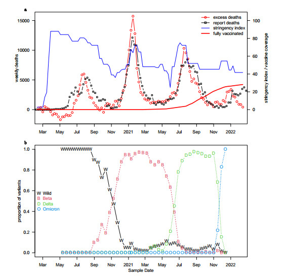
The COVID-19 pandemic caused multiple waves of mortality in South Africa, where three genetic variants of SARS-COV-2 and their ancestral strain dominated consecutively. State-of-the-art mathematical modeling approach was used to estimate the time-varying transmissibility of SARS-COV-2 and the relative transmissibility of Beta, Delta, and Omicron variants. The transmissibility of the three variants were about 73%, 87%, and 276% higher than their preceding variants. To the best of our knowledge, our model is the first simple model that can simulate multiple mortality waves and three variants' replacements in South Africa. The transmissibility of the Omicron variant is substantially higher than that of previous variants.

| [1] |
K. S. S. Abdool, K.Q. Adbool, Omicron SARS-CoV-2 variant: A new chapter in the COVID-19 pandemic. Lancet, 398 (2021), 2126–2128. https://doi.org/10.1016/S0140-6736(21)02758-6 doi: 10.1016/S0140-6736(21)02758-6

|
| [2] |
H. Tegally, E. Wilkinson, C. L. Althaus, M. Giovanetti, J. E. San, J. Giandhari, et al., Rapid replacement of the Beta variant by the Delta variant in South Africa, medRxiv, 2021. https://doi.org/10.1101/2021.09.23.21264018 doi: 10.1101/2021.09.23.21264018
|
| [3] |
S. Cele, I. Gazy, L. Jackson, S.-H. Hwa, H. Tegally, G. Lustig, et al., Escape of SARS-CoV-2 501Y. V2 from neutralization by convalescent plasma, Nature, 593 (2021), 142–146. https://doi.org/10.1038/s41586-021-03471-w doi: 10.1038/s41586-021-03471-w
|
| [4] |
S. A. Madhi, V. Baillie, C. L. Cutland, M. Voysey, A. L. Koen, L. Fairlie, et al., Efficacy of the ChAdOx1 nCoV-19 Covid-19 vaccine against the B. 1.351 variant, N Engl. J. Med., 384 (2021), 1885–1898. https://doi.org/10.1056/NEJMoa2102214 doi: 10.1056/NEJMoa2102214
|
| [5] |
H. Tegally, E. Wikinson, M. Giovanetti, A. Iranzadeh, V. Fonseca, J. Giandhari, et al., Detection of a SARS-CoV-2 variant of concern in South Africa, Nature, 592 (2021), 438–443. https://doi.org/10.1038/s41586-021-03402-9 doi: 10.1038/s41586-021-03402-9
|
| [6] |
H. Chemaitelly, R. Bertollini, L. J. Abu-Raddad, Efficacy of natural immunity against SARS-CoV-2 reinfection with the Beta variant, N Engl. J. Med., 385 (2021), 2585–2586. https://doi.org/10.1056/NEJMc2110300 doi: 10.1056/NEJMc2110300
|
| [7] |
C. Del Rio, P. N. Malani, S. B. Omer, Confronting the delta variant of SARS-CoV-2, summer 2021, JAMA, 326 (2021), 1001–1002. https://doi.org/10.1001/jama.2021.14811 doi: 10.1001/jama.2021.14811
|
| [8] |
Y. Liu, J. Rocklöv, The reproductive number of the Delta variant of SARS-CoV-2 is far higher compared to the ancestral SARS-CoV-2 virus, J. Travel Med., 2021. https://doi.org/10.1093/jtm/taab124 doi: 10.1093/jtm/taab124
|
| [9] |
P. Mlcochova, S. A. Kemp, M. S. Dhar, G. Papa, B. Meng, I. A. T. M. Ferreira, et al., SARS-CoV-2 B. 1.617. 2 Delta variant replication and immune evasion, Nature, 599 (2021), 114–119. https://doi.org/10.1038/s41586-021-03944-y doi: 10.1038/s41586-021-03944-y
|
| [10] | I. Torjesen, Covid-19: Omicron may be more transmissible than other variants and partly resistant to existing vaccines, scientists fear, BMJ. https://doi.org/10.1136/bmj.n2943 |
| [11] |
K. Ito, C. Piantham, H. Nishiura, Predicted dominance of variant Delta of SARS-CoV-2 before Tokyo Olympic Games, Japan, July 2021, Euro. Surveill., 26 (2021), 2100570. https://doi.org/10.2807/1560-7917.ES.2021.26.27.2100570 doi: 10.2807/1560-7917.ES.2021.26.27.2100570
|
| [12] |
H. Gu, P. Krishnan, D. Y. Ng, L. D. J. Chang, G. Y. Z. Liu, S. S. M. Cheng, et al., Probable transmission of SARS-CoV-2 omicron variant in quarantine hotel, Hong Kong, China, November 2021, Emerg. Infect. Dis., 28 (2022), 460. https://doi.org/10.3201/eid2802.212422 doi: 10.3201/eid2802.212422
|
| [13] |
O. Dyer, Covid-19: Peru's official death toll triples to become world's highest, BMJ, 373 (2021), n1442. https://doi.org/10.1136/bmj.n1442 doi: 10.1136/bmj.n1442
|
| [14] |
A. Wilhelm, M. Widera, K. Grikscheit, T. Toptan, B. Schenk, C. Pallas, et al., Reduced neutralization of SARS-CoV-2 omicron variant by vaccine sera and monoclonal antibodies, MedRxiv, 2021. https://doi.org/10.1101/2021.12.07.21267432 doi: 10.1101/2021.12.07.21267432
|
| [15] |
L. Zhang, Q. Li, Z. Liang, T. Li, S. Liu, Q. Q. Cui, et al., The significant immune escape of pseudotyped SARS-CoV-2 Variant Omicron, Emerg. Microbes Infect., 11 (2022), 1–5. https://doi.org/10.1080/22221751.2021.2017757 doi: 10.1080/22221751.2021.2017757
|
| [16] |
W. Dejnirattisai, R. H. Shaw, P. Supasa, C. Liu, A. S. V. Stuart, A. J. Pollard, et al., Reduced neutralisation of SARS-CoV-2 omicron B. 1.1. 529 variant by post-immunisation serum. Lancet, 399 (2022), 234–236. https://doi.org/10.1016/S0140-6736(21)02844-0 doi: 10.1016/S0140-6736(21)02844-0
|
| [17] |
B. J. Gardner, A. M. Kilpatrick, Estimates of reduced vaccine effectiveness against hospitalization, infection, transmission and symptomatic disease of a new SARS-CoV-2 variant, Omicron (B. 1.1. 529), using neutralizing antibody titers, MedRxiv, 2021. https://doi.org/10.1101/2021.12.10.21267594 doi: 10.1101/2021.12.10.21267594
|
| [18] |
C. Kuhlmann, C. K. Mayer, M. Claassen, T. G. Maponga, A. D. Sutherland, T. Suliman, et al., Breakthrough infections with SARS-CoV-2 Omicron variant despite booster dose of mRNA vaccine, Available at SSRN 3981711, 2021. https://dx.doi.org/10.2139/ssrn.3981711 doi: 10.2139/ssrn.3981711
|
| [19] |
H. Nishiura, K. Ito, A. Anzai, T. Kobayashi, C. Piantham, A. J. Rodriguez-Morales, Relative reproduction number of SARS-CoV-2 Omicron (B. 1.1. 529) compared with Delta variant in South Africa, J. Clin. Med., 11 (2021), 30. https://doi.org/10.3390/jcm11010030 doi: 10.3390/jcm11010030
|
| [20] |
Y. Bai, Z. Du, M. Xu, L. Wang, P. Wu, E. H. Y. Lau, et al., International risk of SARS-CoV-2 Omicron variant importations originating in South Africa, medRxiv, 2021. https://doi.org/10.1101/2021.12.07.21267410 doi: 10.1101/2021.12.07.21267410
|
| [21] |
S. Kumar, T. S. Thambiraja, K. Karuppanan, G. Subramaniam, Omicron and Delta variant of SARS‐CoV‐2: a comparative computational study of spike protein. J. Med. Virol., 2021. https://doi.org/10.1002/jmv.27526 doi: 10.1002/jmv.27526
|
| [22] |
J. Chen, R. Wang, N. B. Gilby, G. W. Wei, Omicron (B. 1.1. 529): Infectivity, vaccine breakthrough, and antibody resistance, J. Chem. Inf. Model., 62 (2022), 412–422. https://doi.org/10.1021/acs.jcim.1c01451 doi: 10.1021/acs.jcim.1c01451
|
| [23] |
D. S. Khoury, M. Steain, J. Triccas, A. Sigal, M. P. Davenport, D. Cromer, Analysis: A meta-analysis of Early Results to predict Vaccine efficacy against Omicron, medRxiv, 2021. https://doi.org/10.1101/2021.12.13.21267748 doi: 10.1101/2021.12.13.21267748
|
| [24] |
E. A. Le Rutte, A. J. Shattock, N. Chitnis, S. L. Kelly, M. A. Penny, Assessing impact of Omicron on SARS-CoV-2 dynamics and public health burden, medRxiv, 2021. https://doi.org/10.1101/2021.12.12.21267673 doi: 10.1101/2021.12.12.21267673
|
| [25] | H. Ritchie, E. Mathieu, L. Rodés-Guirao, C. Appel, C. Giattino, E. Ortiz-Ospina, et al., Coronavirus Pandemic (COVID-19), 2020 [cited 2022 Feb 28]. Available from: https://ourworldindata.org/coronavirus |
| [26] |
Y. Shu, J. McCauley, GISAID: Global initiative on sharing all influenza data–from vision to reality, Euro. Surveill., 22 (2017), 30494. https://doi.org/10.2807/1560-7917.ES.2017.22.13.30494 doi: 10.2807/1560-7917.ES.2017.22.13.30494
|
| [27] |
S. Khare, C. Gurry, L. Freitas, M. B. Schultz, G. Bach, A, Diallo, et al., GISAID's Role in Pandemic Response, China CDC Wkly, 3 (2021), 1049. https://doi.org/10.46234/ccdcw2021.255 doi: 10.46234/ccdcw2021.255
|
| [28] |
S. Elbe, G. Buckland‐Merrett, Data, disease and diplomacy: GISAID's innovative contribution to global health, Global Challenges, 1 (2017), 33–46. https://doi.org/10.1002/gch2.1018 doi: 10.1002/gch2.1018
|
| [29] |
E. Mathieu, H. Ritchie, E. Ortiz-Ospina, M. Roser, J. Hasell, C. Appel, et al., A global database of COVID-19 vaccinations, Nat. Hum. Behav., 5 (2021), 947–953. https://doi.org/10.1038/s41562-021-01122-8 doi: 10.1038/s41562-021-01122-8
|
| [30] |
T. Hale, N. Angrist, R. Goldszmidt, B. Kira, A. Petherick, T. Phillips, et al., A global panel database of pandemic policies (Oxford COVID-19 Government Response Tracker), Nat. Hum. Behav., 5 (2021), 529–538. https://doi.org/10.1038/s41562-021-01079-8 doi: 10.1038/s41562-021-01079-8
|
| [31] |
H. Song, G. Fan, S. Zhao, H. Li, Q. Huang, D. He, Forecast of the COVID-19 trend in India: A simple modelling approach, Math. Biosci. Eng., 18 (2021), 9775–9786. https://doi.org/10.3934/mbe.2021479 doi: 10.3934/mbe.2021479
|
| [32] |
H. Song, G. Fan, Y. Liu, X. Wang, D. He, The second wave of COVID-19 in South and Southeast Asia and the effects of vaccination, Front. Med., 8 (2021). https://doi.org/10.3389/fmed.2021.773110 doi: 10.3389/fmed.2021.773110
|
| [33] |
S. S. Musa, X. Wang, S. Zhao, S. Li, N. Hussaini, W. Wang, D. He, The heterogeneous severity of COVID-19 in African countries: A modeling approach, Bull. Math. Biol., 84 (2022), 1–16. https://doi.org/10.1007/s11538-022-00992-x doi: 10.1007/s11538-022-00992-x
|
| [34] |
D. He, E. L. Ionides, A. A. King, Plug-and-play inference for disease dynamics: Measles in large and small populations as a case study, J. R. Soc. Interf., 7 (2010), 271–283. https://doi.org/10.1098/rsif.2009.0151 doi: 10.1098/rsif.2009.0151
|
| [35] |
E. L. Ionides, C. Bretó, A. A. King, Inference for nonlinear dynamical systems, PNAS, 103 (2006), 18438-18443. https://doi.org/10.1073/pnas.0603181103 doi: 10.1073/pnas.0603181103
|
| [36] | W. T. Vetterling, W. H. Press, S. A. Teukolsky, B. P. Flannery, Numerical recipes: Example book C (The Art of Scientific Computing), 1992, Press Syndicate of the University of Cambridge. |
| [37] |
H. Campbell, P. Gustafson, Inferring the COVID-19 IFR with a simple Bayesian evidence synthesis of seroprevalence study data and imprecise mortality data, medRxiv, 2021. https://doi.org/10.1101/2021.05.12.21256975 doi: 10.1101/2021.05.12.21256975
|
| [38] | N. Ferguson, A. Ghani, A. Cori, A. Hogan, W. Hinsley, E. Volz, Report 49: Growth, population distribution and immune escape of Omicron in England, Imperial College London. https://doi.org/10.25561/93038 |
| [39] |
K. Leung, M. H. Shum, G. M. Leung, T. T. Lam, J. T. Wu, Early transmissibility assessment of the N501Y mutant strains of SARS-CoV-2 in the United Kingdom, October to November 2020, Euro. Surveill., 26 (2021), 2002106. https://doi.org/10.2807/1560-7917.ES.2020.26.1.2002106 doi: 10.2807/1560-7917.ES.2020.26.1.2002106
|
| [40] |
B. Roquebert, S. Trombert-Paolantoni, S. Haim-Boukobza, E. Lecorche, L. Verdurme, V. Foulongne, et al., The SARS-CoV-2 B. 1.351 lineage (VOC β) is outgrowing the B. 1.1. 7 lineage (VOC α) in some French regions in April 2021, Euro. Surveill., 26 (2021), 2100447. https://doi.org/10.2807/1560-7917.ES.2021.26.23.2100447 doi: 10.2807/1560-7917.ES.2021.26.23.2100447
|
| [41] |
K. Ito, C. Piantham, H. Nishiura, Relative instantaneous reproduction number of Omicron SARS‐CoV‐2 variant with respect to the Delta variant in Denmark, J. Med. Virol., 94 (2022), 2265–2268. https://doi.org/10.1002/jmv.27560 doi: 10.1002/jmv.27560
|
| [42] |
Y. M. Chu, A. Ali, M. A. Khan, S. Islam, S. Ullah, Dynamics of fractional order COVID-19 model with a case study of Saudi Arabia, Results Phys., 21 (2021), 103787. https://doi.org/10.1016/j.rinp.2020.103787 doi: 10.1016/j.rinp.2020.103787
|
| [43] |
X. P. Li, Y. Wang, M. A. Khan, M. Y. Alshahrani, T. Muhammad, A dynamical study of SARS-COV-2: A study of third wave, Results Phys., 29 (2021), 104705. https://doi.org/10.1016/j.rinp.2021.104705 doi: 10.1016/j.rinp.2021.104705
|


Figures(3) / Tables(1)

Yangyang Yu, Yuan Liu, Shi Zhao, Daihai He. A simple model to estimate the transmissibility of the Beta, Delta, and Omicron variants of SARS-COV-2 in South Africa[J]. Mathematical Biosciences and Engineering, 2022, 19(10): 10361-10373. doi: 10.3934/mbe.2022485


 DownLoad: