Determination of the location of the needle entry point based on an improved pruning algorithm

Guangyuan Zhang; Xiaonan Gao; Zhenfang Zhu; Fengyv Zhou; Dexin Yu; Guangyuan Zhang; Xiaonan Gao; Zhenfang Zhu; Fengyv Zhou; Dexin Yu

doi:10.3934/mbe.2022372

Mathematical Biosciences and Engineering

2022, Volume 19, Issue 8: 7952-7977. doi: 10.3934/mbe.2022372

Previous Article Next Article

Research article Special Issues

Determination of the location of the needle entry point based on an improved pruning algorithm

1.
School of Information Science and Electrical Engineering, Shan Dong Jiao Tong University, Jinan 250000, China
2.
School of Control Science and Engineering, Shandong University, Jinan 250000, China
3.
Department of Radiology, Qilu Hospital of Shandong University, Jinan 250000, China

Academic Editor: Biswajeet Pradhan

Received: 23 January 2022 Revised: 04 May 2022 Accepted: 16 May 2022 Published: 30 May 2022

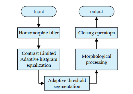
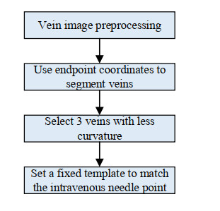
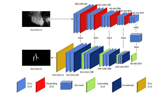
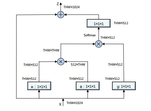
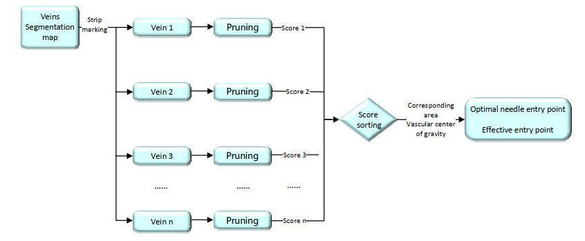
Since the emergence of new coronaviruses and their variant virus, a large number of medical resources around the world have been put into treatment. In this case, the purpose of this article is to develop a handback intravenous intelligence injection robot, which reduces the direct contact between medical staff and patients and reduces the risk of infection. The core technology of hand back intravenous intelligent robot is a handlet venous vessel detection and segmentation and the position of the needle point position decision. In this paper, an image processing algorithm based on U-Net improvement mechanism (AT-U-Net) is proposed for core technology. It is investigated using a self-built dorsal hand vein database and the results show that it performs well, with an F1-score of 93.91%. After the detection of a dorsal hand vein, this paper proposes a location decision method for the needle entry point based on an improved pruning algorithm (PT-Pruning). The extraction of the trunk line of the dorsal hand vein is realized through this algorithm. Considering the vascular cross-sectional area and bending of each vein injection point area, the optimal injection point of the dorsal hand vein is obtained via a comprehensive decision-making process. Using the self-built dorsal hand vein injection point database, the accuracy of the detection of the effective injection area reaches 96.73%. The accuracy for the detection of the injection area at the optimal needle entry point is 96.50%, which lays a foundation for subsequent mechanical automatic injection.
- image processing,
- dorsal hand vein,
- automatic injection,
- needle entry point,
- location decision
Citation: Guangyuan Zhang, Xiaonan Gao, Zhenfang Zhu, Fengyv Zhou, Dexin Yu. Determination of the location of the needle entry point based on an improved pruning algorithm[J]. Mathematical Biosciences and Engineering, 2022, 19(8): 7952-7977. doi: 10.3934/mbe.2022372

Related Papers:

Abstract

Since the emergence of new coronaviruses and their variant virus, a large number of medical resources around the world have been put into treatment. In this case, the purpose of this article is to develop a handback intravenous intelligence injection robot, which reduces the direct contact between medical staff and patients and reduces the risk of infection. The core technology of hand back intravenous intelligent robot is a handlet venous vessel detection and segmentation and the position of the needle point position decision. In this paper, an image processing algorithm based on U-Net improvement mechanism (AT-U-Net) is proposed for core technology. It is investigated using a self-built dorsal hand vein database and the results show that it performs well, with an F1-score of 93.91%. After the detection of a dorsal hand vein, this paper proposes a location decision method for the needle entry point based on an improved pruning algorithm (PT-Pruning). The extraction of the trunk line of the dorsal hand vein is realized through this algorithm. Considering the vascular cross-sectional area and bending of each vein injection point area, the optimal injection point of the dorsal hand vein is obtained via a comprehensive decision-making process. Using the self-built dorsal hand vein injection point database, the accuracy of the detection of the effective injection area reaches 96.73%. The accuracy for the detection of the injection area at the optimal needle entry point is 96.50%, which lays a foundation for subsequent mechanical automatic injection.

References

[1]	Y. Wu, Investigation on infection prevention and control needs of frontline medical staff in fever clinic during epidemic period of COVID-19, Health Educ. Health Promot. , 16 (2021), 90-92. https://doi.org/10.16117/j.cnki.31-1974/r.202101090 doi: 10.16117/j.cnki.31-1974/r.202101090
[2]	R. Deng, F. Chen, S. S. Liu, L. Yuan, J. P. Song, Influencing factors for psychological stress of health care workers in COVID-19 isolation wards, Chin. J. Infect. Control, 19 (2020), 256-261. https://doi.org/10.12138/j.issn.1671-9638.20206395 doi: 10.12138/j.issn.1671-9638.20206395
[3]	J. M. Leipheimer, M. L. Balter, A. I. Chen, E. J. Pantin, A. E. Davidovich, K. S. Labazzo, et al., First-in-human evaluation of a hand-held automated venipuncture device for rapid venous blood draws, Technology, 7 (2019), 98-107. https://doi.org/10.1142/S2339547819500067 doi: 10.1142/S2339547819500067
[4]	Guangming Daily, Tongji University: "Contactless" Automatic Needle and Blood Collection Robot was Invented, 2021. Available form: https://news.gmw.cn/2021-01/31/content_34586222.htm.
[5]	N. Takahashi, T. Dohi, H. Endo, M. Takeuchi, S. Doi, Y. Kato, et al., Coronary lipid-rich plaque characteristics in Japanese patients with acute coronary syndrome and stable angina: A near infrared spectroscopy and intravascular ultrasound study, IJC Heart Vasculature, 33 (2021), 100747. https://doi.org/10.1016/j.ijcha.2021.100747 doi: 10.1016/j.ijcha.2021.100747
[6]	Y. Zhao, Z. Li, H. Tang, S. Lin, W. Zeng, D. Ye, et al., [Mn(PaPy2Q)(NO)]ClO4, a near-infrared light activated release of nitric oxide drug as a nitric oxide donor for therapy of human prostate cancer cells in vitro and in vivo, Biomed. Pharmacother. , 137 (2021), 111388. https://doi.org/10.1016/j.biopha.2021.111388 doi: 10.1016/j.biopha.2021.111388
[7]	S. Kitahara, Y. Kataoka, H. Miura, T. Nishii, K. Nishimura, Kota Murai, et al., The feasibility and limitation of coronary computed tomographic angiography imaging to identify coronary lipid-rich atheroma in vivo: Findings from near-infrared spectroscopy analysis, Atherosclerosis, 322 (2021), 1-7. https://doi.org/10.1016/j.atherosclerosis.2021.02.019 doi: 10.1016/j.atherosclerosis.2021.02.019
[8]	Y. L. Katsogridakis, R. Seshadri, C. Sullivan, M. L. Waltzman, Veinlite transillumination in the pediatric emergency department: A therapeutic interventional trial, Pediatr. Emerg. Care, 24 (2008), 83-88. https://doi.org/10.1097/PEC.0b013e318163db5f doi: 10.1097/PEC.0b013e318163db5f
[9]	T. Y. Xu, X. W. Hui, S. Lin, A near infrared finger vein recognition approach based on wavelet grayscale surface matching, Adv. Lasers Optoelectron. , 53 (2016), 9. https://doi.org/10.3788/LOP53.041005 doi: 10.3788/LOP53.041005
[10]	E. Ostańska, D. Aebisher, D. Bartusik-Aebisher, The potential of photodynamic therapy in current breast cancer treatment methodologies, Biomed. Pharmacother. , 137 (2021), 111302. https://doi.org/10.1016/j.biopha.2021.111302 doi: 10.1016/j.biopha.2021.111302
[11]	J. Dong, Design and experiment of the prototype of the intravenous blood collection robot principle, Ph. D thesis, Harbin Institute of Technology, 2020.
[12]	X. Zhang, Y. H. Guo, G. Li, J. L. He, Image automatic recognition and mark of hand vein injection parts, Infrared Technol. , 37 (2015), 5.
[13]	O. Ronneberger, P. Fischer, T. Brox, U-Net: Convolutional networks for biomedical image segmentation, in International Conference on Medical Image Computing and Computer-assisted Intervention, (2015), 234-241. https://doi.org/10.1007/978-3-319-24574-4_28
[14]	J. Le'Clerc Arrastia, N. Heilenkötter, D. Otero Baguer, L. Hauberg-Lotte, T. Boskamp, et al., Deeply supervised UNet for semantic segmentation to assist dermatopathological assessment of basal cell carcinoma, J. Imaging, 7 (2021), 71. https://doi.org/10.3390/jimaging7040071 doi: 10.3390/jimaging7040071
[15]	K. B. Soulami, N. Kaabouch, M. N. Saidi, A. Tamtaoui, Breast cancer: One-stage automated detection, segmentation, and classification of digital mammograms using UNet model based-semantic segmentation, Biomed. Signal Process. Control, 66 (2021), 102481. https://doi.org/10.1016/j.bspc.2021.102481 doi: 10.1016/j.bspc.2021.102481
[16]	D. T. Kushnure, S. N. Talbar, MS-UNet: A multi-scale UNet with feature recalibration approach for automatic liver and tumor segmentation in CT images, Comput. Med. Imaging Graphics, 89 (2021), 101885. https://doi.org/10.1016/j.compmedimag.2021.101885 doi: 10.1016/j.compmedimag.2021.101885
[17]	E. Thomas, S. J. Pawan, S. Kumar, A. Horo, S. Niyas, S. Vinayagamani, et al., Multi-res-attention UNet: A CNN model for the segmentation of focal cortical dysplasia lesions from magnetic resonance images, IEEE J. Biomed. Health Inf. , 25 (2020), 1724-1734. https://doi.org/10.1109/JBHI.2020.3024188 doi: 10.1109/JBHI.2020.3024188
[18]	Y. Zhang, J. Wu, Y. Liu, Y. Chen, E. X. Wu, X. Tang, MI-UNet: multi-inputs UNet incorporating brain parcellation for stroke lesion segmentation from T1-weighted magnetic resonance images, IEEE J. Biomed. Health Inf. , 25 (2020), 526-535. https://doi.org/10.1109/JBHI.2020.2996783 doi: 10.1109/JBHI.2020.2996783
[19]	J. J. Zhao, X. Xiong, L. Zhang, T. Fu, D. X, Zhao, An image enhancement algorithm for dorsal veins of the hand based on CLAHE and top-hat transforms, Laser Infrared, 39 (2009), 3.
[20]	D. M. Zhang, Low-quality Finger Vein Images Enhanced, Ph. D thesis, Chongqing University of Technology, 2011.
[21]	N. Miura, A. Nagasaka, T. Miyatake, Extraction of finger-vein patterns using maximum curvature points in image profiles, Ice Trans. Inf. Syst. , 90 (2007), 1185-1194. https://doi.org/10.1093/ietisy/e90-d.8.1185 doi: 10.1093/ietisy/e90-d.8.1185
[22]	S. Wang, J. Chen, Y. Lu, COVID-19 chest CT image segmentation based on federated learning and blockchain, J. Jilin Univ. Eng. Edition, 51 (2021), 10.
[23]	J. He, Q. Zhu, K. Zhang, P. Yu, J. Tang, An evolvable adversarial network with gradient penalty for COVID-19 infection segmentation, 113 (2021), 107947. https://doi.org/10.1016/j.asoc.2021.107947
[24]	J. Wang, Y. Jiang, M. Li, N. Wang, B. Cui, W. Liu, Effects of qingre huoxue jiedu formula on nerve growth factor-induced psoriasis., Chin. J. Integr. Med. , 28 (2022), 236-242. https://doi.org/10.1007/s11655-021-3493-4 doi: 10.1007/s11655-021-3493-4
[25]	C. Zhao, Y. Xu, Z. He, J. Tang, Y. Zhang, J. Han, et al., Lung segmentation and automatic detection of COVID-19 using radiomic features from chest CT images, Pattern Recognit. , 119 (2021), 108071. https://doi.org/10.1016/j.patcog.2021.108071 doi: 10.1016/j.patcog.2021.108071
[26]	Y. Cheng, M. Ma, L. Zhang, C. J. Jin, L. Ma, Y. Zhou, Retinal blood vessel segmentation based on densely connected U-Net, Math. Biosci. Eng. , 17 (2020), 3088-3108. https://doi.org/10.3934/mbe.2020175 doi: 10.3934/mbe.2020175
[27]	X. Deng, Y. Liu, H. Chen, Three-dimensional image reconstruction based on improved U-net network for anatomy of pulmonary segmentectomy, Math. Biosci. Eng. , 18 (2021), 3313-3322. https://doi.org/10.3934/mbe.2021165 doi: 10.3934/mbe.2021165
[28]	N. Sheng, D. Liu, J. Zhang, C. Che, J. Zhang, Second-order ResU-Net for automatic MRI brain tumor segmentation, Math. Biosci. Eng. , 18 (2021), 4943-4960. https://doi.org/10.3934/mbe.2021251 doi: 10.3934/mbe.2021251
[29]	J. Yang, M. Fu, Y. Hu, Liver vessel segmentation based on inter-scale V-Net, Math. Biosci. Eng. , 18 (2021), 4327-4340. https://doi.org/10.3934/mbe.2021217 doi: 10.3934/mbe.2021217
[30]	L. Li, C. Li, L. Li, Y. Tang, Q. Yang, An integrated approach for remanufacturing job shop scheduling with routing alternatives, Math. Biosci. Eng. , 16 (2019), 2063-2085. https://doi.org/10.3934/mbe.2019101 doi: 10.3934/mbe.2019101
[31]	Y Liu, N Qi, Q Zhu, W Li, CR-U-Net: Cascaded U-Net with residual mapping for liver segmentation in CT images, in 2019 IEEE Visual Communications and Image Processing (VCIP) IEEE, 2019. https://doi.org/10.1109/VCIP47243.2019.8966072
[32]	Q. Cai, Y. Liu, R. Zhang, Two-stage retinal vascular segmentation based on improved U-Net, Adv. Lasers Optoelectron., 58 (2021), 1617002. https://doi.org/10.3788/LOP202158.1617002 doi: 10.3788/LOP202158.1617002
[33]	C. E. He, H. J. Xu, Z. Wang, L. P. Ma, Research on multimodal magnetic resonance brain tumor image automatic segmentation algorithm, Acta Optica Sinica, 40 (2020), 66-75.
[34]	H. Huang, C. Peng, R. Y. Wu, J. L. Tao, J. Q. Zhang, Self-supervised transfer learning of lung nodule classification based on partially annotated CT images, Acta Optica Sinica, 40 (2020), 99-106. https://doi.org/10.3788/AOS202040.1810003 doi: 10.3788/AOS202040.1810003
[35]	L. Wang, C. X. Chen, X. Fu, L. Wang, Vascular segmentation of retinal images of preterm infants based on FDMU-net, Adv. Lasers Optoelectron. , 58 (2021), 475-481.
[36]	W Zhang, Z Zhu, Y Zhang, Cell image segmentation method based on residual block and attention mechanism, Acta Optica Sinica, 40 (2020), 76-83.
[37]	X. Wang, R. Girshick, A. Gupta, K. He, Non-local neural networks, in Proceedings of the IEEE Conference on Computer Vision and Pattern Recognition, (2018), 7797-7803.
[38]	W. X. Liu, Z. X. Wang, G. G. Mu, Ridge tracing and application in post-processing of thinned figerprints, J. Optoelectron. Lasers, 2 (2002), 184-187.
[39]	W. Wang, Using UNet and PSPNet to explore the reusability principle of CNN parameters, preprint, arXiv: 2008.03414.
[40]	H. Zhao, J. Shi, X. Qi, X. Wang, J. Jia, Pyramid scene parsing network, in Proceedings of the IEEE Conference on Computer Vision and Pattern Recognition, (2017), 2881-2890.
[41]	J. Zhou, M. Hao, D. Zhang, P. Zou, W. Zhang, Fusion PSPnet image segmentation based method for multi-focus image fusion, IEEE Photonics J., 11 (2019), 1-12. https://doi.org/10.1109/JPHOT.2019.2950949 doi: 10.1109/JPHOT.2019.2950949
[42]	V. Badrinarayanan, A. Kendall, SegNet: A deep convolutional encoder-decoder architecture for image segmentation, IEEE Trans. Pattern Anal. Machine Intell., 39 (2017), 2481-2495. https://doi.org/10.1109/TPAMI.2016.2644615 doi: 10.1109/TPAMI.2016.2644615
[43]	G. Lin, A. Milan, C. Shen, I. Reid, Refinenet: Multi-path refinement networks for high-resolution semantic segmentation, in Proceedings of the IEEE Conference on Computer Vision and Pattern Rrecognition, (2017), 1925-1934.
[44]	R. Y. Zhou, W. Z. Shen, PI-Unet: Study of heterogeneous iris precise segmentation neural network model, Comput. Eng. Appl., 57 (2021), 7. https://doi.org/10.3778/j.issn.1002-8331.2005-0068 doi: 10.3778/j.issn.1002-8331.2005-0068

Reader Comments

Your name:*

Email:*
© 2022 the Author(s), licensee AIMS Press. This is an open access article distributed under the terms of the Creative Commons Attribution License (http://creativecommons.org/licenses/by/4.0)