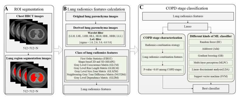
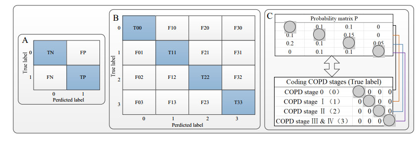
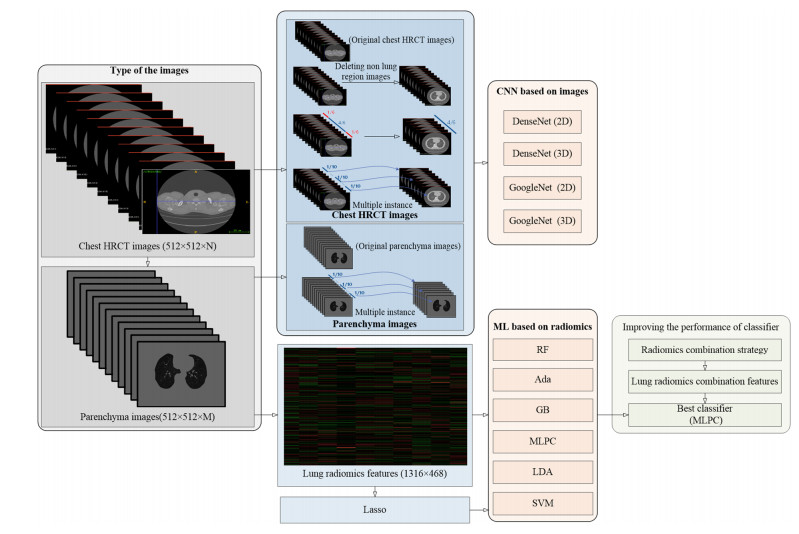
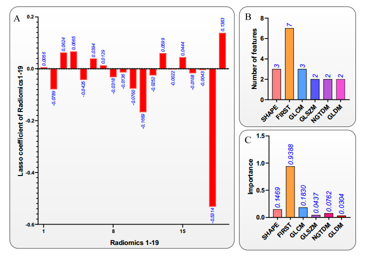
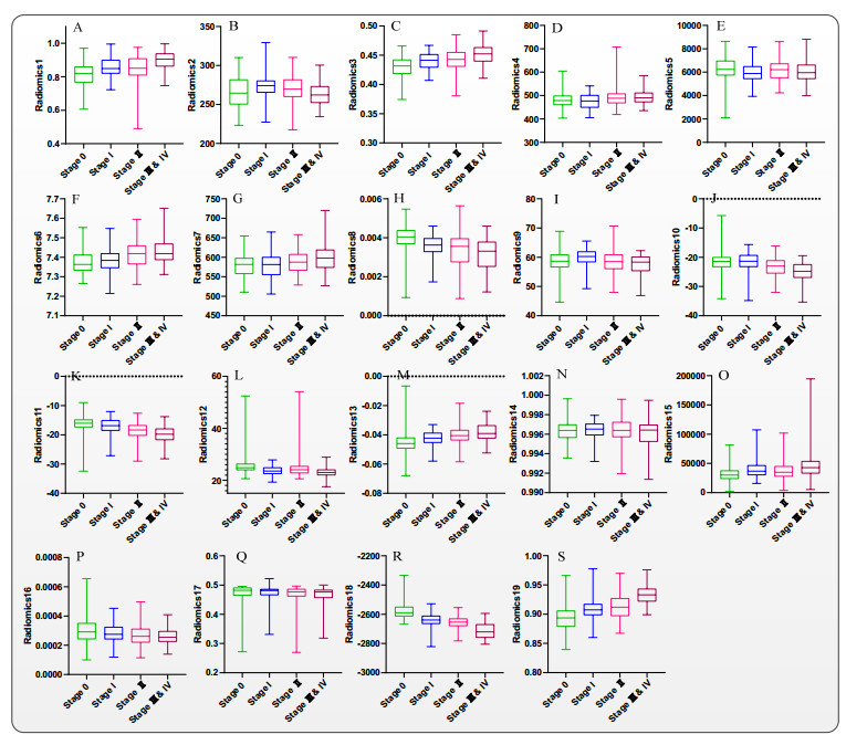
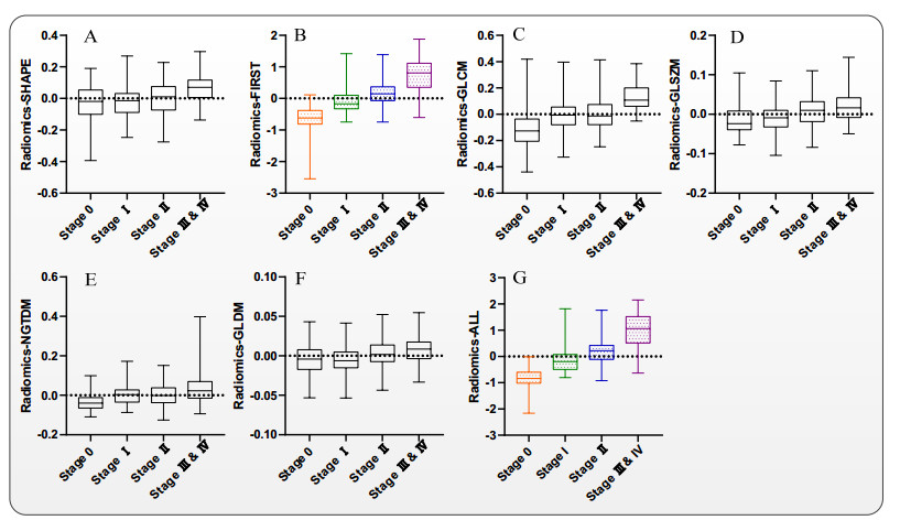
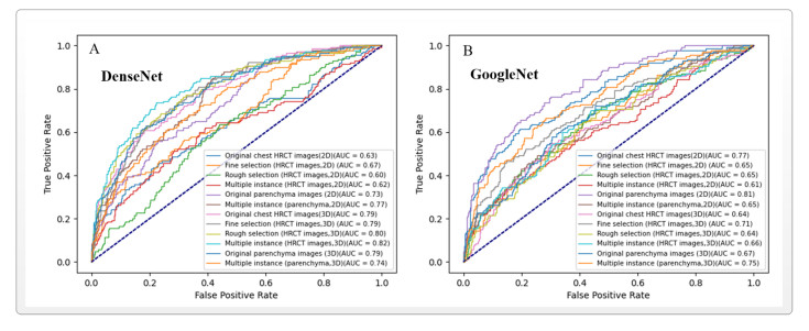
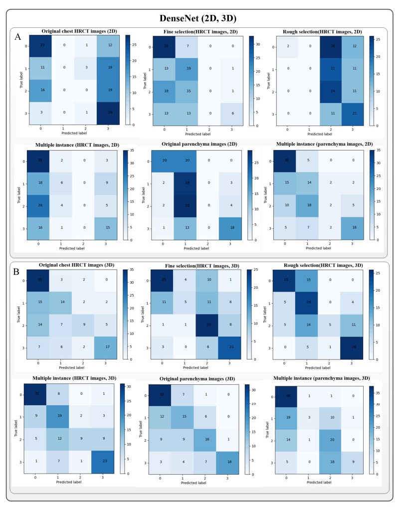
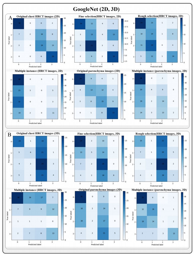
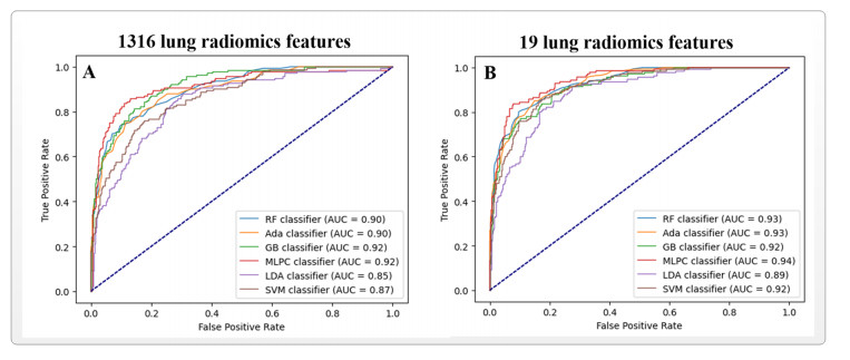
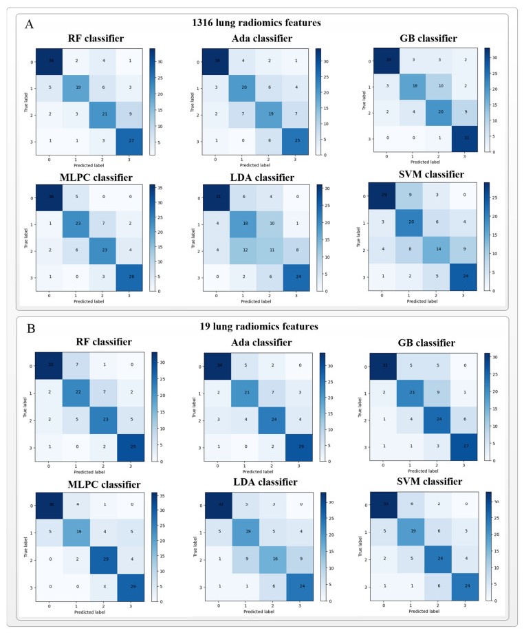
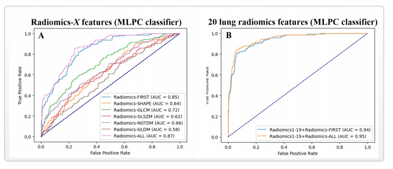
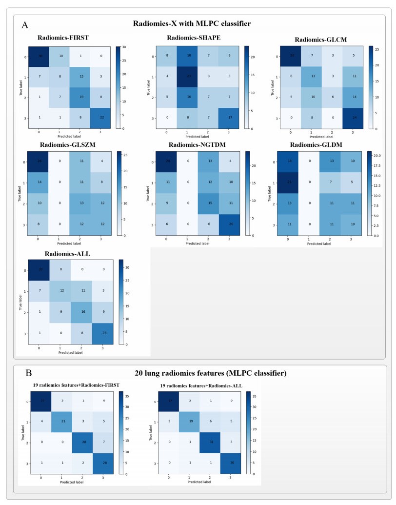
Computed tomography (CT) has been the most effective modality for characterizing and quantifying chronic obstructive pulmonary disease (COPD). Radiomics features extracted from the region of interest in chest CT images have been widely used for lung diseases, but they have not yet been extensively investigated for COPD. Therefore, it is necessary to understand COPD from the lung radiomics features and apply them for COPD diagnostic applications, such as COPD stage classification. Lung radiomics features are used for characterizing and classifying the COPD stage in this paper. First, 19 lung radiomics features are selected from 1316 lung radiomics features per subject by using Lasso. Second, the best performance classifier (multi-layer perceptron classifier, MLP classifier) is determined. Third, two lung radiomics combination features, Radiomics-FIRST and Radiomics-ALL, are constructed based on 19 selected lung radiomics features by using the proposed lung radiomics combination strategy for characterizing the COPD stage. Lastly, the 19 selected lung radiomics features with Radiomics-FIRST/Radiomics-ALL are used to classify the COPD stage based on the best performance classifier. The results show that the classification ability of lung radiomics features based on machine learning (ML) methods is better than that of the chest high-resolution CT (HRCT) images based on classic convolutional neural networks (CNNs). In addition, the classifier performance of the 19 lung radiomics features selected by Lasso is better than that of the 1316 lung radiomics features. The accuracy, precision, recall, F1-score and AUC of the MLP classifier with the 19 selected lung radiomics features and Radiomics-ALL were 0.83, 0.83, 0.83, 0.82 and 0.95, respectively. It is concluded that, for the chest HRCT images, compared to the classic CNN, the ML methods based on lung radiomics features are more suitable and interpretable for COPD classification. In addition, the proposed lung radiomics combination strategy for characterizing the COPD stage effectively improves the classifier performance by 12% overall (accuracy: 3%, precision: 3%, recall: 3%, F1-score: 2% and AUC: 1%).
Citation: Yingjian Yang, Wei Li, Yingwei Guo, Nanrong Zeng, Shicong Wang, Ziran Chen, Yang Liu, Huai Chen, Wenxin Duan, Xian Li, Wei Zhao, Rongchang Chen, Yan Kang. Lung radiomics features for characterizing and classifying COPD stage based on feature combination strategy and multi-layer perceptron classifier[J]. Mathematical Biosciences and Engineering, 2022, 19(8): 7826-7855. doi: 10.3934/mbe.2022366
Computed tomography (CT) has been the most effective modality for characterizing and quantifying chronic obstructive pulmonary disease (COPD). Radiomics features extracted from the region of interest in chest CT images have been widely used for lung diseases, but they have not yet been extensively investigated for COPD. Therefore, it is necessary to understand COPD from the lung radiomics features and apply them for COPD diagnostic applications, such as COPD stage classification. Lung radiomics features are used for characterizing and classifying the COPD stage in this paper. First, 19 lung radiomics features are selected from 1316 lung radiomics features per subject by using Lasso. Second, the best performance classifier (multi-layer perceptron classifier, MLP classifier) is determined. Third, two lung radiomics combination features, Radiomics-FIRST and Radiomics-ALL, are constructed based on 19 selected lung radiomics features by using the proposed lung radiomics combination strategy for characterizing the COPD stage. Lastly, the 19 selected lung radiomics features with Radiomics-FIRST/Radiomics-ALL are used to classify the COPD stage based on the best performance classifier. The results show that the classification ability of lung radiomics features based on machine learning (ML) methods is better than that of the chest high-resolution CT (HRCT) images based on classic convolutional neural networks (CNNs). In addition, the classifier performance of the 19 lung radiomics features selected by Lasso is better than that of the 1316 lung radiomics features. The accuracy, precision, recall, F1-score and AUC of the MLP classifier with the 19 selected lung radiomics features and Radiomics-ALL were 0.83, 0.83, 0.83, 0.82 and 0.95, respectively. It is concluded that, for the chest HRCT images, compared to the classic CNN, the ML methods based on lung radiomics features are more suitable and interpretable for COPD classification. In addition, the proposed lung radiomics combination strategy for characterizing the COPD stage effectively improves the classifier performance by 12% overall (accuracy: 3%, precision: 3%, recall: 3%, F1-score: 2% and AUC: 1%).

| [1] |
A. G. Mathioudakis, G. A. Mathioudakis, The phenotypes of chronic obstructive pulmonary disease, Arch. Hellenic Med., 31 (2014), 558-569. https://doi.org/10.1080/15412550701629663 doi: 10.1080/15412550701629663

|
| [2] | GOLD 2022: Global initiative for chronic obstructive lung disease, 2022. |
| [3] |
D. A. Suffredini, R. M. Reed, At the twisted heart of nicotine addiction, BMJ Case Rep., 2012. https://doi.org/10.1136/bcr-2012-006240 doi: 10.1136/bcr-2012-006240
|
| [4] |
P. W. Jones, Health status measurement in chronic obstructive pulmonary disease, Thorax, 56 (2001). https://doi.org/10.1201/9780203913406-14 doi: 10.1201/9780203913406-14
|
| [5] |
C. D. Brown, J. O. Benditt, F. C. Sciurba, S. M. Lee, G. J. Criner, Z. Mosenifar, et al., Exercise testing in severe emphysema: association with quality of life and lung function, COPD J. Chron. Obstruct. Pulm. Dis., 5 (2008), 117-124. https://doi.org/10.1080/15412550801941265 doi: 10.1080/15412550801941265
|
| [6] |
D. A. Lynch, Progress in Imaging COPD, 2004-2014, Chron. Obstruct. Pulm. Dis.: J. COPD Found., 1 (2014), 73-82. https://doi.org/10.15326/jcopdf.1.1.2014.0125 doi: 10.15326/jcopdf.1.1.2014.0125
|
| [7] |
P. J. Castaldi, R. S. J. Estépar, C. S. Mendoza, C. P. Hersh, N. Laird, J. D. Crapo, et al., Distinct quantitative computed tomography emphysema patterns are associated with physiology and function in smokers, Am. J. Respir. Crit. Care Med., 188 (2013), 1083-1090. https://doi.org/10.1164/rccm.201305-0873oc doi: 10.1164/rccm.201305-0873oc
|
| [8] |
T. B. Grydeland, A. Dirksen, H. O. Coxson, T. M. Eagan, E. Thorsen, S. G. Pillai, et al., Quantitative computed tomography measures of emphysema and airway wall thickness are related to respiratory symptoms, Am. J. Respir. Crit. Care Med., 181 (2010), 353-359. https://doi.org/10.1164/rccm.200907-1008oc doi: 10.1164/rccm.200907-1008oc
|
| [9] |
V. Kim, A. Davey, A. P. Comellas, M. K. Han, G. Washko, C. H. Martinez, et al., Clinical and computed tomographic predictors of chronic bronchitis in COPD: a cross Sectional analysis of the COPDGene study, Respir. Res., 15 (2014), 1-9. https://doi.org/10.1186/1465-9921-15-52 doi: 10.1186/1465-9921-15-52
|
| [10] |
S. P. Bhatt, N. L. Terry, H. Nath, J. A. Zach, J. Tschirren, M. S. Bolding, et al., Association between expiratory central airway collapse and respiratory outcomes among smokers, Jama, 315 (2016), 498-505. https://doi.org/10.1164/rccm.202008-3122le doi: 10.1164/rccm.202008-3122le
|
| [11] |
C. P. Hersh, G. R. Washko, R. S. J. Estépar, S. Lutz, P. J. Friedman, M. K. Han, et al., Paired inspiratory-expiratory chest CT scans to assess for small airways disease in COPD, Respir. Res., 14 (2013), 1-11. https://doi.org/10.1164/ajrccm-conference.2012.185.1_meetingabstracts.a6539 doi: 10.1164/ajrccm-conference.2012.185.1_meetingabstracts.a6539
|
| [12] |
S. Bodduluri, J. M. Reinhardt, E. A. Hoffman, J. D. Newell Jr, H. Nath, M. T. Dransfield, et al., Signs of gas trapping in normal lung density regions in smokers, Am. J. Respir. Crit. Care Med., 196 (2017), 1404-1410. https://doi.org/10.1164/rccm.201705-0855oc doi: 10.1164/rccm.201705-0855oc
|
| [13] |
C. J. Galbán, M. K. Han, J. L. Boes, K. A. Chughtai, C. R. Meyer, T. D. Johnson, et al. Computed tomography-based biomarker provides unique signature for diagnosis of COPD phenotypes and disease progression, Nat. Med., 18 (2012), 1711-1715. https://doi.org/10.1038/nm.2971 doi: 10.1038/nm.2971
|
| [14] |
S. Bodduluri, S. P. Bhatt, E. A. Hoffman, J. D. Newell, C. H. Martinez, M. T. Dransfield, et al., Biomechanical CT metrics are associated with patient outcomes in COPD, Thorax, 72 (2017), 409-414. https://doi.org/10.1136/thoraxjnl-2016-209544 doi: 10.1136/thoraxjnl-2016-209544
|
| [15] |
S. P. Bhatt, S. Bodduluri, E. A. Hoffman, J. D. Newell Jr, J. C. Sieren, M. T. Dransfield, et al., Computed tomography measure of lung at risk and lung function decline in chronic obstructive pulmonary disease, Am. J. Respir. Crit. Care Med., 196 (2017), 569-576. https://doi.org/10.1164/rccm.201701-0050oc doi: 10.1164/rccm.201701-0050oc
|
| [16] |
G. R. Washko, G. L. Kinney, J. C. Ross, R. S. J. Estépar, M. K. Han, M. T. Dransfield, et al., Lung Mass in Smokers, Acad. Radiol., 24 (2016), 386-392. https://doi.org/10.1016/j.acra.2016.10.011 doi: 10.1016/j.acra.2016.10.011
|
| [17] |
J. M. Wells, G. R. Washko, M. K. Han, N. Abbas, H. Nath, A. J. Mamary, et al., Pulmonary arterial enlargement and acute exacerbations of COPD, N. Engl. J. Med., 367 (2012), 913-921. https://doi.org/10.1136/thoraxjnl-2013-203397 doi: 10.1136/thoraxjnl-2013-203397
|
| [18] |
R. S. J. Estépar, G. L. Kinney, J. L. Black-Shinn, R. P. Bowler, G. L. Kindlmann, J. C. Ross, et al., Computed tomographic measures of pulmonary vascular morphology in smokers and their clinical implications, Am. J. Respir. Crit. Care Med., 188 (2013), 231-239. https://doi.org/10.1164/rccm.201301-0162oc doi: 10.1164/rccm.201301-0162oc
|
| [19] |
P. Lambin, E. Rios-Velazquez, R. Leijenaar, S. Carvalho, R. G. Van Stiphout, P. Granton, et al., Radiomics: Extracting more information from medical images using advanced feature analysis, Eur. J. Cancer, 43 (2007), 441-446. https://doi.org/10.1016/j.ejca.2011.11.036 doi: 10.1016/j.ejca.2011.11.036
|
| [20] |
A. N. Frix, F. Cousin, T. Refaee, F. Bottari, A. Vaidyanathan, C. Desir, et al., Radiomics in lung diseases imaging: State-of-the-art for clinicians, J. Pers. Med., 11 (2021), 1-20. https://doi.org/10.3390/jpm11070602 doi: 10.3390/jpm11070602
|
| [21] |
S. M. Rezaeijo, R. Abedi-Firouzjah, M. Ghorvei, S. Sarnameh, Screening of COVID-19 based on the extracted radiomics features from chest CT images, J. X-Ray Sci. Technol., 29 (2021), 1-15. https://doi.org/10.3233/xst-200831 doi: 10.3233/xst-200831
|
| [22] |
F. Xiao, R. Sun, W. Sun, D. Xu, L. Lan, H. Li, et al., Radiomics analysis of chest CT to predict the overall survival for the severe patients of COVID-19 pneumonia, Phys. Med. Biol., 66 (2021), 1-11. https://doi.org/10.1088/1361-6560/abf717 doi: 10.1088/1361-6560/abf717
|
| [23] |
F. Xiong, Y. Wang, T. You, H. Li, T. Fu, H. Tan, et al., The clinical classification of patients with COVID-19 pneumonia was predicted by Radiomics using chest CT, Medicine, 100 (2021), 1-8. https://doi.org/10.1097/md.0000000000025307 doi: 10.1097/md.0000000000025307
|
| [24] |
M. Tamal, M. Alshammari, M. Alabdullah, R. Hourani, H. A. Alola, T. M. Hegazi, An integrated framework with machine learning and radiomics for accurate and rapid early diagnosis of COVID-19 from chest x-ray, Expert Syst. Appl., 180 (2021), 1-8. https://doi.org/10.1101/2020.10.01.20205146 doi: 10.1101/2020.10.01.20205146
|
| [25] |
Y. Tang, T. Zhang, X. Zhou, Y. Zhao, H. Xu, Y. Liu, et al., The preoperative prognostic value of the radiomics nomogram based on CT combined with machine learning in patients with intrahepatic cholangiocarcinoma, World J. Surg. Oncol., 19 (2021), 1-13. https://doi.org/10.1186/s12957-021-02162-0 doi: 10.1186/s12957-021-02162-0
|
| [26] |
X. Han, J. Yang, J. Luo, P. Chen, Z. Zhang, A. Alu, et al., Application of CT-based radiomics in discriminating pancreatic cystadenomas from pancreatic neuroendocrine tumors using machine learning methods, Front. Oncol., 11 (2021), 1-13. https://doi.org/10.3389/fonc.2021.606677 doi: 10.3389/fonc.2021.606677
|
| [27] | M. F. A. Chaudhary, E. A. Hoffman, A. P. Comellas, J. Guo, S. Fortis, S. Bodduluri, et al., CT texture features predict severe COPD exacerbations in spiromics, in American Thoracic Society 2021 International Conference, (2021), 1122-1122. https://doi.org/10.1164/ajrccm-conference.2021.203.1_meetingabstracts.a1122 |
| [28] |
M. Occhipinti, M. Paoletti, B. J. Bartholmai, S. Rajagopalan, R. A. Karwoski, C. Nardi, et al., Spirometric assessment of emphysema presence and severity as measured by quantitative CT and CT-based radiomics in COPD, Respir. Res., 20 (2019), 1-11. https://doi.org/10.1186/s12931-019-1049-3 doi: 10.1186/s12931-019-1049-3
|
| [29] |
G. Wu, A. Ibrahim, I. Halilaj, R. T. Leijenaar, W. Rogers, H. A. Gietema, et al., The emerging role of radiomics in COPD and lung cancer, Respiration, 99 (2020), 99-107. https://doi.org/10.1159/000505429 doi: 10.1159/000505429
|
| [30] |
G. Maragatham, S. Rajendran, Improving the classifier accuracy with an integrated approach using medical data-a study, Int. J. Med. Eng. Inf., 12 (2020), 313-321. https://doi.org/10.1504/ijmei.2020.10029317 doi: 10.1504/ijmei.2020.10029317
|
| [31] |
D. Lu, Q. Weng, A survey of image classification methods and techniques for improving classification performance, Int. J. Remote Sens., 28 (2007), 823-870. https://doi.org/10.1080/01431160600746456 doi: 10.1080/01431160600746456
|
| [32] |
R. C. Au, W. C. Tan, J. Bourbeau, J. C. Hogg, M. Kirby, Impact of image pre-processing methods on computed tomography radiomics features in chronic obstructive pulmonary disease, Phys. Med. Biol., 66 (2021). https://doi.org/10.2139/ssrn.3349696 doi: 10.2139/ssrn.3349696
|
| [33] |
J. Yun, Y. H. Cho, S. M. Lee, J. Hwang, J. S. Lee, Y. M. Oh, et al., Deep radiomics-based survival prediction in patients with chronic obstructive pulmonary disease, Sci. Rep., 11 (2021), 1-9. https://doi.org/10.1038/s41598-021-94535-4 doi: 10.1038/s41598-021-94535-4
|
| [34] | R. C. Au, W. C. Tan, J. Bourbeau, J. C. Hogg, M. Kirby, Radiomics Analysis to Predict Presence of Chronic Obstructive Pulmonary Disease and Symptoms Using Machine Learning, in TP121 COPD: FROM CELLS TO THE CLINIC, American Thoracic Society, 2021. https://doi.org/10.1164/ajrccm-conference.2021.203.1_meetingabstracts.a4568 |
| [35] | C. Liang, J. Xu, F. Wang, H. Chen, J. Tang, D. Chen, et al., Development of a radiomics model for predicting COPD exacerbations based on complementary visual information, in TP041 DIAGNOSIS AND RISK ASSESSMENT IN COPD, American Thoracic Society, 2021. https://doi.org/10.1164/ajrccm-conference.2021.203.1_meetingabstracts.a2296 |
| [36] |
Y. Yang, W. Li, Y. Guo, Y. Liu, Q. Li, K. Yang, et al., Early COPD risk decision for adults aged from 40 to 79 years based on lung radiomics features, Front. Med., 9 (2022), 1-15. https://doi.org/10.3389/fmed.2022.845286 doi: 10.3389/fmed.2022.845286
|
| [37] |
Y. Yang, W. Li, Y. Kang, Y. Guo, K. Yang, Q. Li, et al., A novel lung radiomics feature for characterizing resting heart rate and COPD stage evolution based on radiomics feature combination strategy, Math. Biosci. Eng., 19 (2022), 4145-4165. https://doi.org/10.3934/mbe.2022191 doi: 10.3934/mbe.2022191
|
| [38] |
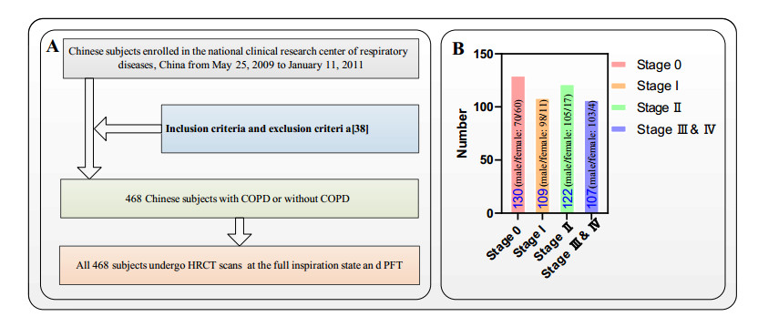
Y. Zhou, P. L. Bruijnzeel, C. McCrae, J. Zheng, U. Nihlen, R. Zhou, et al., Study on risk factors and phenotypes of acute exacerbations of chronic obstructive pulmonary disease in Guangzhou, China-design and baseline characteristics, J. Thorac. Dis., 7 (2015), 720-733. https://doi:10.3978/j.issn.2072-1439.2015.04.14 doi: 10.3978/j.issn.2072-1439.2015.04.14
|
| [39] |
J. Hofmanninger, F. Prayer, J. Pan, S. Rohrich, H. Prosch, G. Langs, Automatic lung segmentation in routine imaging is a data diversity problem, not a methodology problem, Eur. Radiol. Exp., 4 (2020), 1-13. https://doi.org/10.1186/s41747-020-00173-2 doi: 10.1186/s41747-020-00173-2
|
| [40] |
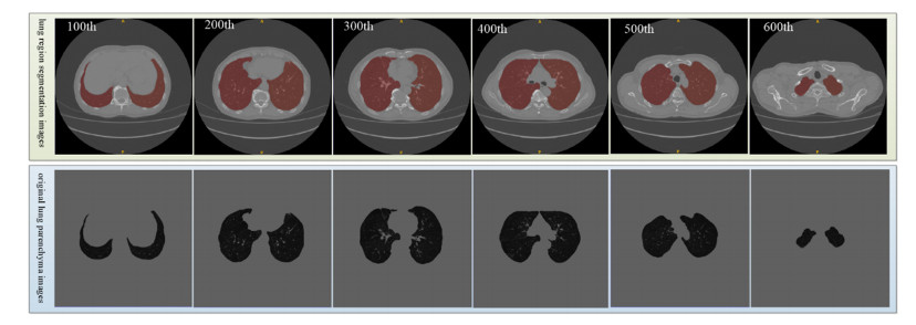
Y. Yang, Q. Li, Y. Guo, Y. Liu, X. Li, J. Guo, et al., Lung parenchyma parameters measure of rats from pulmonary window computed tomography images based on ResU-Net model for medical respiratory researches, Math. Biosci. Eng., 18 (2021), 4193-4211. https://doi.org/10.3934/mbe.2021210 doi: 10.3934/mbe.2021210
|
| [41] | Y. Yang, Y. Guo, J. Guo, Y. Gao, Y. Kang, A method of abstracting single pulmonary lobe from computed tomography pulmonary images for locating COPD, in Proceedings of the Fourth International Conference on Biological Information and Biomedical Engineering, (2020), 1-6. https://doi.org/10.1145/3403782.3403805 |
| [42] |
J. J. M. van Griethuysen, A. Fedorov, C. Parmar, A. Hosny, N. Aucoin, V. Narayan, et al., Computational radiomics system to decode the radiographic phenotype, Cancer Res., 77 (2017), 104-107. https://doi.org/10.1158/0008-5472.can-17-0339 doi: 10.1158/0008-5472.can-17-0339
|
| [43] |
R. Tibshirani, Regression shrinkage and selection via the Lasso, J. R. Stat. Soc. B, 58 (2007), 267-288. https://doi.org/10.1111/j.2517-6161.1996.tb02080.x doi: 10.1111/j.2517-6161.1996.tb02080.x
|
| [44] |
N. Simon, J. Friedman, T. Hastie, R. Tibshirani, Regularization paths for Cox's proportional hazards model via coordinate descent, J. Stat. Software, 39 (2011), 1-13. https://doi.org/10.18637/jss.v039.i05 doi: 10.18637/jss.v039.i05
|
| [45] | Y. Qi, Random forest for bioinformatics, in Ensemble machine learning: methods and applications, Springer, Boston, MA, (2012), 307-323. https://doi.org/10.1007/978-1-4419-9326-7_11 |
| [46] | T. H. Kim, D. C. Park, D. M. Woo, T. Jeong, S. Y. Min, Multi-class classifier-based adaboost algorithm, in International conference on intelligent science and intelligent data engineering, Springer, Berlin, Heidelberg, (2011), 122-127. https://doi.org/10.1007/978-3-642-31919-8_16 |
| [47] | V. K. Ayyadevara, Gradient boosting machine, in Pro machine learning algorithms, Apress, Berkeley, CA, (2018), 117-134. https://doi.org/10.1007/978-1-4842-3564-5_6 |
| [48] |
M. Taki, A. Rohani, F. Soheili-Fard, A. Abdeshahi, Assessment of energy consumption and modeling of output energy for wheat production by neural network (MLP and RBF) and Gaussian process regression (GPR) models, J. Cleaner Prod. 172 (2018), 3028-3041. https://doi.org/10.1016/j.jclepro.2017.11.107 doi: 10.1016/j.jclepro.2017.11.107
|
| [49] |
W. Hu, W. Hu, S. Maybank, Adaboost-based algorithm for network intrusion detection, IEEE Trans. Syst. Man Cybern. Part B Cybern., 38 (2008), 577-583. https://doi.org/10.1109/tsmcb.2007.914695 doi: 10.1109/tsmcb.2007.914695
|
| [50] | S. Suthaharan, Support vector machine, in Machine learning models and algorithms for big data classification, Springer, Boston, MA, (2016), 207-235. https://doi.org/10.1007/978-1-4899-7641-3_9 |
| [51] |
Q. Li, Y. Yang, Y. Guo, W. Li, Y. Liu, H. Liu, et al., Performance evaluation of deep learning classification network for image features, IEEE Access, 9 (2021), 9318-9333. https://doi.org/10.1109/access.2020.3048956 doi: 10.1109/access.2020.3048956
|
| [52] |
M. A. Carbonneau, V. Cheplygina, E. Granger, G. Gagnon, Multiple instance learning: A survey of problem characteristics and applications, Pattern Recognit., 77 (2018), 329-353. https://doi.org/10.1016/j.patcog.2017.10.009 doi: 10.1016/j.patcog.2017.10.009
|
| [53] |
H. Polat, H. D. Mehr, Classification of pulmonary CT images by using hybrid 3D-deep convolutional neural network architecture, Appl. Sci., 9 (2019), 1-15. https://doi.org/10.3390/app9050940 doi: 10.3390/app9050940
|
| [54] |
A. Chon, N. Balachandar, P. Lu, Deep convolutional neural networks for lung cancer detection, Standford Univ., (2017), 1-9. https://doi.org/10.1109/uemcon47517.2019.8993023 doi: 10.1109/uemcon47517.2019.8993023
|
| [55] |
S. P. Singh, L. Wang, S. Gupta, H. Goli, P. Padmanabhan, B. Gulyás, 3D deep learning on medical images: a review, Sensors, 20 (2020), 1-24. https://doi.org/10.3390/s20185097 doi: 10.3390/s20185097
|
| [56] |
B. H. Lee, D. H. Oh, T. Y. Kim, 3D Virtual reality game with deep learning-based hand gesture recognition, J. Korea Comput. Graphics Soc., 24 (2018), 41-48. https://doi.org/10.15701/kcgs.2018.24.5.41 doi: 10.15701/kcgs.2018.24.5.41
|
| [57] |
B. George, S. Seals, I. Aban, Survival analysis and regression models, J. Nucl. Cardiol., 21 (2014), 686-694. https://doi.org/10.1007/s12350-014-9908-2 doi: 10.1007/s12350-014-9908-2
|
| [58] | L. Torrey, J. Shavlik, Transfer learning, in Handbook of research on machine learning applications and trends: algorithms, methods, and techniques, IGI global, (2010), 242-264. https://doi.org/10.4018/978-1-60566-766-9.ch011 |
Figures(15) / Tables(12)

Yingjian Yang, Wei Li, Yingwei Guo, Nanrong Zeng, Shicong Wang, Ziran Chen, Yang Liu, Huai Chen, Wenxin Duan, Xian Li, Wei Zhao, Rongchang Chen, Yan Kang. Lung radiomics features for characterizing and classifying COPD stage based on feature combination strategy and multi-layer perceptron classifier[J]. Mathematical Biosciences and Engineering, 2022, 19(8): 7826-7855. doi: 10.3934/mbe.2022366


 DownLoad: