Salp swarm algorithm (SSA) is a recently proposed, powerful swarm-intelligence based optimizer, which is inspired by the unique foraging style of salps in oceans. However, the original SSA suffers from some limitations including immature balance between exploitation and exploration operators, slow convergence and local optimal stagnation. To alleviate these deficiencies, a modified SSA (called VC-SSA) with velocity clamping strategy, reduction factor tactic, and adaptive weight mechanism is developed. Firstly, a novel velocity clamping mechanism is designed to boost the exploitation ability and the solution accuracy. Next, a reduction factor is arranged to bolster the exploration capability and accelerate the convergence speed. Finally, a novel position update equation is designed by injecting an inertia weight to catch a better balance between local and global search. 23 classical benchmark test problems, 30 complex optimization tasks from CEC 2017, and five engineering design problems are employed to authenticate the effectiveness of the developed VC-SSA. The experimental results of VC-SSA are compared with a series of cutting-edge metaheuristics. The comparisons reveal that VC-SSA provides better performance against the canonical SSA, SSA variants, and other well-established metaheuristic paradigms. In addition, VC-SSA is utilized to handle a mobile robot path planning task. The results show that VC-SSA can provide the best results compared to the competitors and it can serve as an auxiliary tool for mobile robot path planning.
Citation: Hongwei Ding, Xingguo Cao, Zongshan Wang, Gaurav Dhiman, Peng Hou, Jie Wang, Aishan Li, Xiang Hu. Velocity clamping-assisted adaptive salp swarm algorithm: balance analysis and case studies[J]. Mathematical Biosciences and Engineering, 2022, 19(8): 7756-7804. doi: 10.3934/mbe.2022364
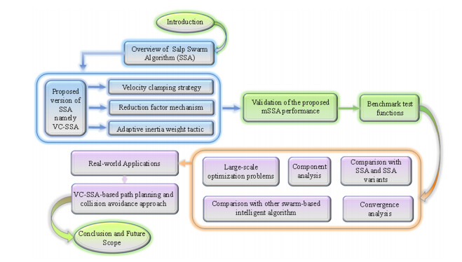
Salp swarm algorithm (SSA) is a recently proposed, powerful swarm-intelligence based optimizer, which is inspired by the unique foraging style of salps in oceans. However, the original SSA suffers from some limitations including immature balance between exploitation and exploration operators, slow convergence and local optimal stagnation. To alleviate these deficiencies, a modified SSA (called VC-SSA) with velocity clamping strategy, reduction factor tactic, and adaptive weight mechanism is developed. Firstly, a novel velocity clamping mechanism is designed to boost the exploitation ability and the solution accuracy. Next, a reduction factor is arranged to bolster the exploration capability and accelerate the convergence speed. Finally, a novel position update equation is designed by injecting an inertia weight to catch a better balance between local and global search. 23 classical benchmark test problems, 30 complex optimization tasks from CEC 2017, and five engineering design problems are employed to authenticate the effectiveness of the developed VC-SSA. The experimental results of VC-SSA are compared with a series of cutting-edge metaheuristics. The comparisons reveal that VC-SSA provides better performance against the canonical SSA, SSA variants, and other well-established metaheuristic paradigms. In addition, VC-SSA is utilized to handle a mobile robot path planning task. The results show that VC-SSA can provide the best results compared to the competitors and it can serve as an auxiliary tool for mobile robot path planning.

| [1] |
F. Cicirelli, A. Forestiero, A Giordano, C. Mastroianni, Transparent and efficient parallelization of swarm algorithms, ACM Trans. Auton. Adapt. Syst., 11 (2016), 1-26. https://doi.org/10.1145/2897373 doi: 10.1145/2897373

|
| [2] |
A. M. Lal, S. M. Anouncia, Modernizing the multi-temporal multispectral remotely sensed image change detection for global maxima through binary particle swarm optimization, J. King Saud Univ., Comput. Inf. Sci., 34 (2022), 95-103. https://doi.org/10.1016/j.jksuci.2018.10.010 doi: 10.1016/j.jksuci.2018.10.010
|
| [3] |
A. Faramarzi, M. Heidarinejad, S. Mirjalili, A. H. Gandomi, Marine predators algorithm: A nature-inspired metaheuristic, Expert Syst. Appl., 152 (2020), 113377. https://doi.org/10.1016/j.eswa.2020.113377 doi: 10.1016/j.eswa.2020.113377
|
| [4] |
D. Sarkar, S. Choudhury, A. Majumder, Enhanced-Ant-AODV for optimal route selection in mobile ad-hoc network, J. King Saud Univ., Comput. Inf. Sci., 33 (2021), 1186-1201. https://doi.org/10.1016/j.jksuci.2018.08.013 doi: 10.1016/j.jksuci.2018.08.013
|
| [5] |
G. G. Wang, S. Deb, L. D. S. Coelho, Earthworm optimisation algorithm: a bio-inspired metaheuristic algorithm for global optimisation problems, Int. J. Bio-Inspired Comput., 12 (2018), 1-22. https://doi.org/10.1504/IJBIC.2018.093328 doi: 10.1504/IJBIC.2018.093328
|
| [6] |
D. Karaboga, B. Basturk, A powerful and efficient algorithm for numerical function optimization: artificial bee colony (ABC) algorithm, J. Global Optim., 39 (2007), 459-471. https://doi.org/10.1007/s10898-007-9149-x doi: 10.1007/s10898-007-9149-x
|
| [7] |
Z. Wang, H. Ding, B. Li, L. Bao, Z. Yang, An energy efficient routing protocol based on improved artificial bee colony algorithm for wireless sensor networks, IEEE Access, 8 (2020), 133577-133596. https://doi.org/10.1109/ACCESS.2020.3010313 doi: 10.1109/ACCESS.2020.3010313
|
| [8] |
S. Mirjalili, Moth-flame optimization algorithm: A novel nature-inspired heuristic paradigm, Knowl.-Based Syst., 89 (2015), 228-249. https://doi.org/10.1016/j.knosys.2015.07.006 doi: 10.1016/j.knosys.2015.07.006
|
| [9] | X. S. Yang, Firefly algorithm, in Engineering Optimization: An Introduction with Metaheuristic Applications, (2010), 221-230. https://doi.org/10.1002/9780470640425.ch17 |
| [10] |
Z. Wang, H. Ding, B. Li, L. Bao, Z. Yang, Q. Liu, Energy efficient cluster based routing protocol for WSN using firefly algorithm and ant colony optimization, Wireless Pers. Commun., 2022. https://doi.org/10.1007/s11277-022-09651-9 doi: 10.1007/s11277-022-09651-9
|
| [11] |
S. Mirjalili, A. Lewis, The whale optimization algorithm, Adv. Eng. Software, 95 (2016), 51-67. https://doi.org/10.1016/j.advengsoft.2016.01.008 doi: 10.1016/j.advengsoft.2016.01.008
|
| [12] |
X. S. Yang, S. Deb, Cuckoo search: recent advances and applications, Neural Comput. Appl., 24 (2014), 169-174. https://doi.org/10.1007/s00521-013-1367-1 doi: 10.1007/s00521-013-1367-1
|
| [13] |
S. Mirjalili, S. M. Mirjalili, A. Lewis, Grey wolf optimizer, Adv. Eng. Software, 69 (2014), 46-61. https://doi.org/10.1016/j.advengsoft.2013.12.007 doi: 10.1016/j.advengsoft.2013.12.007
|
| [14] |
K. P. B. Resma, M. S. Nair, Multilevel thresholding for image segmentation using Krill Herd Optimization algorithm, J. King Saud Univ., Comput. Inf. Sci., 33 (2021), 528-541. https://doi.org/10.1016/j.jksuci.2018.04.007 doi: 10.1016/j.jksuci.2018.04.007
|
| [15] |
A. A. Heidari, S. Mirjalili, H. Faris, I. Aljarah, M. Mafarja, H. Chen, Harris hawks optimization: Algorithm and applications, Future Gener. Comput. Syst., 97 (2019), 849-872. https://doi.org/10.1016/j.future.2019.02.028 doi: 10.1016/j.future.2019.02.028
|
| [16] |
G. G. Wang, S. Deb, Z. Cui, Monarch butterfly optimization, Neural Comput. Appl., 31 (2019), 1995-2014. https://doi.org/10.1007/s00521-015-1923-y doi: 10.1007/s00521-015-1923-y
|
| [17] |
S. Saremi, S. Mirjalili, A. Lewis, Grasshopper optimisation algorithm: theory and application, Adv. Eng. Software, 105 (2017), 30-47. https://doi.org/10.1016/j.advengsoft.2017.01.004 doi: 10.1016/j.advengsoft.2017.01.004
|
| [18] |
W. Li, G. G.Wang, A. H. Alavi, Learning-based elephant herding optimization algorithm for solving numerical optimization problems, Knowl.-Based Syst., 195 (2020), 105675. https://doi.org/10.1016/j.knosys.2020.105675 doi: 10.1016/j.knosys.2020.105675
|
| [19] |
S. Li, H. Chen, M. Wang, A. A. Heidari, S. Mirjalili, Slime mould algorithm: A new method for stochastic optimization, Future Gener. Comput. Syst., 111 (2020), 300-323. https://doi.org/10.1016/j.future.2020.03.055 doi: 10.1016/j.future.2020.03.055
|
| [20] |
Y. Yang, H. Chen, A. A. Heidari, A. H. Gandomi, Hunger games search: Visions, conception, implementation, deep analysis, perspectives, and towards performance shifts, Expert Syst. Appl., 177 (2021), 114864. https://doi.org/10.1016/j.eswa.2021.114864 doi: 10.1016/j.eswa.2021.114864
|
| [21] |
I. Ahmadianfar, A. A. Heidari, A. H. Gandomi, X. Chu, H. Chen, RUN beyond the metaphor: An efficient optimization algorithm based on Runge Kutta method, Expert Syst. Appl., 181 (2021), 115079. https://doi.org/10.1016/j.eswa.2021.115079 doi: 10.1016/j.eswa.2021.115079
|
| [22] |
J. Tu, H. Chen, M. Wang, A. H. Gandomi, The colony predation algorithm, J. Bionic Eng., 18 (2021), 674-710. https://doi.org/10.1007/s42235-021-0050-y doi: 10.1007/s42235-021-0050-y
|
| [23] |
I. Ahmadianfar, A. A. Heidari, S. Noshadian, H. Chen, A. H. Gandomi, INFO: An efficient optimization algorithm based on weighted mean of vectors, Expert Syst. Appl., 195 (2022), 116516. https://doi.org/10.1016/j.eswa.2022.116516 doi: 10.1016/j.eswa.2022.116516
|
| [24] |
S. Mirjalili, A. H. Gandomi, S. Z. Mirjalili, S. Saremi, H. Faris, S. M. Mirjalili, Salp swarm algorithm: A bio-inspired optimizer for engineering design problems, Adv. Eng. Software, 114 (2017), 163-191. https://doi.org/10.1016/j.advengsoft.2017.07.002 doi: 10.1016/j.advengsoft.2017.07.002
|
| [25] |
Z. Wang, H. Ding, Z. Yang, B. Li, Z. Guan, L. Bao, Rank-driven salp swarm algorithm with orthogonal opposition-based learning for global optimization, Appl. Intell., 52 (2022), 7922-7964. https://doi.org/10.1007/s10489-021-02776-7 doi: 10.1007/s10489-021-02776-7
|
| [26] |
A. A. Ewees, M. A. Al-qaness, M. Abd Elaziz, Enhanced salp swarm algorithm based on firefly algorithm for unrelated parallel machine scheduling with setup times, Appl. Math. Modell., 94 (2021), 285-305. https://doi.org/10.1016/j.apm.2021.01.017 doi: 10.1016/j.apm.2021.01.017
|
| [27] |
Q. Tu, Y. Liu, F. Han, X. Liu, Y. Xie, Range-free localization using reliable anchor pair selection and quantum-behaved salp swarm algorithm for anisotropic wireless sensor networks, Ad Hoc Networks, 113 (2021), 102406. https://doi.org/10.1016/j.adhoc.2020.102406 doi: 10.1016/j.adhoc.2020.102406
|
| [28] |
M. Tubishat, N. Idris, L. Shuib, M. A. Abushariah, S. Mirjalili, Improved salp swarm algorithm based on opposition based learning and novel local search algorithm for feature selection, Expert Syst. Appl., 145 (2020), 113122. https://doi.org/10.1016/j.eswa.2019.113122 doi: 10.1016/j.eswa.2019.113122
|
| [29] |
B. Nautiyal, R. Prakash, V. Vimal, G. Liang, H. Chen, Improved salp swarm algorithm with mutation schemes for solving global optimization and engineering problems, Eng. Comput., 2021. https://doi.org/10.1007/s00366-020-01252-z doi: 10.1007/s00366-020-01252-z
|
| [30] |
M. M. Saafan, E. M. El-Gendy, IWOSSA: An improved whale optimization salp swarm algorithm for solving optimization problems, Expert Syst. Appl., 176 (2021), 114901. https://doi.org/10.1016/j.eswa.2021.114901 doi: 10.1016/j.eswa.2021.114901
|
| [31] |
D. Bairathi, D. Gopalani, An improved salp swarm algorithm for complex multi-modal problems, Soft Comput., 25 (2021), 10441-10465. https://doi.org/10.1007/s00500-021-05757-7 doi: 10.1007/s00500-021-05757-7
|
| [32] |
E. Çelik, N. Öztürk, Y. Arya, Advancement of the search process of salp swarm algorithm for global optimization problems, Expert Syst. Appl., 182 (2021), 115292. https://doi.org/10.1016/j.eswa.2021.115292 doi: 10.1016/j.eswa.2021.115292
|
| [33] |
Q. Zhang, Z. Wang, A. A. Heidari, W. Gui, Q. Shao, H. Chen, et al., Gaussian barebone salp swarm algorithm with stochastic fractal search for medical image segmentation: a COVID-19 case study, Comput. Biol. Med., 139 (2021), 104941. https://doi.org/10.1016/j.compbiomed.2021.104941 doi: 10.1016/j.compbiomed.2021.104941
|
| [34] |
H. Zhang, T. Liu, X. Ye, A. A. Heidari, G. Liang, H. Chen, et al., Differential evolution-assisted salp swarm algorithm with chaotic structure for real-world problems, Eng. Comput., 2022. https://doi.org/10.1007/s00366-021-01545-x doi: 10.1007/s00366-021-01545-x
|
| [35] |
S. Zhao, P. Wang, X. Zhao, H. Tuiabieh, M. Mafarja, H. Chen, Elite dominance scheme ingrained adaptive salp swarm algorithm: a comprehensive study, Eng. Comput., 2021. https://doi.org/10.1007/s00366-021-01464-x doi: 10.1007/s00366-021-01464-x
|
| [36] |
J. Song, C. Chen, A. A. Heidari, J. Liu, H. Yu, H. Chen, Performance optimization of annealing salp swarm algorithm: frameworks and applications for engineering design, J. Comput. Des. Eng., 9 (2022), 633-669. https://doi.org/10.1093/jcde/qwac021 doi: 10.1093/jcde/qwac021
|
| [37] |
S. Zhao, P. Wang, A. A. Heidari, H. Chen, W. He, S. Xu, Performance optimization of salp swarm algorithm for multi-threshold image segmentation: Comprehensive study of breast cancer microscopy, Comput. Biol. Med., 139 (2021), 105015. https://doi.org/10.1016/j.compbiomed.2021.105015 doi: 10.1016/j.compbiomed.2021.105015
|
| [38] |
D. H. Wolpert, W. G. Macready, No free lunch theorems for optimization, IEEE Trans. Evol. Comput., 1 (1997), 67-82. https://doi.org/10.1109/4235.585893 doi: 10.1109/4235.585893
|
| [39] |
J. J. Jena, S. C. Satapathy, A new adaptive tuned Social Group Optimization (SGO) algorithm with sigmoid-adaptive inertia weight for solving engineering design problems, Multimed Tools Appl., 2021. https://doi.org/10.1007/s11042-021-11266-4 doi: 10.1007/s11042-021-11266-4
|
| [40] |
A. Naik, S. C. Satapathy, A. S. Ashour, N. Dey, Social group optimization for global optimization of multimodal functions and data clustering problems, Neural Comput. Appl., 30 (2018), 271-287. https://doi.org/10.1007/s00521-016-2686-9 doi: 10.1007/s00521-016-2686-9
|
| [41] |
P. Sun, H. Liu, Y. Zhang, L. Tu, Q. Meng, An intensify atom search optimization for engineering design problems, Appl. Math. Modell., 89 (2021), 837-859. https://doi.org/10.1016/j.apm.2020.07.052 doi: 10.1016/j.apm.2020.07.052
|
| [42] |
W. Zhao, L. Wang, Z. Zhang, Atom search optimization and its application to solve a hydrogeologic parameter estimation problem, Knowl.-Based Syst., 163 (2019), 283-304. https://doi.org/10.1016/j.knosys.2018.08.030 doi: 10.1016/j.knosys.2018.08.030
|
| [43] |
L. Ma, C. Wang, N. Xie, M. Shi, Y. Ye, L. Wang, Moth-flame optimization algorithm based on diversity and mutation strategy, Appl. Intell., 51 (2021), 5836-5872. https://doi.org/10.1007/s10489-020-02081-9 doi: 10.1007/s10489-020-02081-9
|
| [44] |
Y. Li, Y. Zhao, J. Liu, Dynamic sine cosine algorithm for large-scale global optimization problems, Expert Syst. Appl., 177 (2021), 114950. https://doi.org/10.1016/j.eswa.2021.114950 doi: 10.1016/j.eswa.2021.114950
|
| [45] |
S. Mirjalili, SCA: A sine cosine algorithm for solving optimization problems, Knowl.-Based Syst., 96 (2016), 120-133. https://doi.org/10.1016/j.knosys.2015.12.022 doi: 10.1016/j.knosys.2015.12.022
|
| [46] |
W. Long, J. Jiao, X. Liang, T. Wu, M. Xu, S. Cai, Pinhole-imaging-based learning butterfly optimization algorithm for global optimization and feature selection, Appl. Soft Comput., 103 (2021), 107146. https://doi.org/10.1016/j.asoc.2021.107146 doi: 10.1016/j.asoc.2021.107146
|
| [47] |
R. Salgotra, U. Singh, S. Singh, G. Singh, N. Mittal, Self-adaptive salp swarm algorithm for engineering optimization problems, Appl. Math. Modell., 89 (2021), 188-207. https://doi.org/10.1016/j.apm.2020.08.014 doi: 10.1016/j.apm.2020.08.014
|
| [48] |
H. Ren, J. Li, H. Chen, C. Li, Stability of salp swarm algorithm with random replacement and double adaptive weighting, Appl. Math. Modell., 95 (2021), 503-523. https://doi.org/10.1016/j.apm.2021.02.002 doi: 10.1016/j.apm.2021.02.002
|
| [49] |
G. I. Sayed, G. Khoriba, M. H. Haggag, A novel chaotic salp swarm algorithm for global optimization and feature selection, Appl. Intell., 48 (2018), 3462-3481. https://doi.org/10.1007/s10489-018-1158-6 doi: 10.1007/s10489-018-1158-6
|
| [50] |
M. H. Qais, H. M. Hasanien, S. Alghuwainem, Enhanced salp swarm algorithm: application to variable speed wind generators, Eng. Appl. Artif. Intell., 80 (2019), 82-96. https://doi.org/10.1016/j.engappai.2019.01.011 doi: 10.1016/j.engappai.2019.01.011
|
| [51] |
M. Braik, A. Sheta, H. Turabieh, H. Alhiary, A novel lifetime scheme for enhancing the convergence performance of salp swarm algorithm, Soft Comput., 25 (2021), 181-206. https://doi.org/10.1007/s00500-020-05130-0 doi: 10.1007/s00500-020-05130-0
|
| [52] |
A. G. Hussien, An enhanced opposition-based salp swarm algorithm for global optimization and engineering problems, J. Ambient Intell. Humaniz. Comput., 13 (2022), 129-150. https://doi.org/10.1007/s12652-021-02892-9 doi: 10.1007/s12652-021-02892-9
|
| [53] |
F. A. Ozbay, B. Alatas, Adaptive salp swarm optimization algorithms with inertia weights for novel fake news detection model in online social media, Multimedia Tools Appl., 80 (2021), 34333-34357. https://doi.org/10.1007/s11042-021-11006-8 doi: 10.1007/s11042-021-11006-8
|
| [54] |
S. Kaur, L. K. Awasthi, A. L. Sangal, G. Dhiman, Tunicate swarm algorithm: a new bio-inspired based metaheuristic paradigm for global optimization, Eng. Appl. Artif. Intell., 90 (2020), 103541. https://doi.org/10.1016/j.engappai.2020.103541 doi: 10.1016/j.engappai.2020.103541
|
| [55] |
S. Dhargupta, M. Ghosh, S. Mirjalili, R. Sarkar, Selective opposition based grey wolf optimization, Expert Syst. Appl., 151 (2020), 113389. https://doi.org/10.1016/j.eswa.2020.113389 doi: 10.1016/j.eswa.2020.113389
|
| [56] |
A. Faramarzi, M. Heidarinejad, B. Stephens, S. Mirjalili, Equilibrium optimizer: A novel optimization algorithm, Knowl.-Based Syst., 191 (2020), 105190. https://doi.org/10.1016/j.knosys.2019.105190 doi: 10.1016/j.knosys.2019.105190
|
| [57] |
L. Abualigah, A. Diabat, S. Mirjalili, M. A. Elaziz, A. H. Gandomi, The arithmetic optimization algorithm, Comput. Methods Appl. Mech. Eng., 376 (2021), 113609. https://doi.org/10.1016/j.cma.2020.113609 doi: 10.1016/j.cma.2020.113609
|
| [58] |
F. A. Hashim, K. Hussain, E. H. Houssein, M. S. Mabrouk, W. Al-Atabany, Archimedes optimization algorithm: a new metaheuristic algorithm for solving optimization problems, Appl. Intell., 51 (2021), 1531-1551. https://doi.org/10.1007/s10489-020-01893-z doi: 10.1007/s10489-020-01893-z
|
| [59] |
M. H. Nadimi-Shahraki, S. Taghian, S. Mirjalili, An improved grey wolf optimizer for solving engineering problems, Expert Syst. Appl., 166 (2021), 113917. https://doi.org/10.1016/j.eswa.2020.113917 doi: 10.1016/j.eswa.2020.113917
|
| [60] |
W. Shan, Z. Qiao, A. A. Heidari, H. Chen, H. Turabieh, Y. Teng, Double adaptive weights for stabilization of moth flame optimizer: balance analysis, engineering cases, and medical diagnosis, Knowl.-Based Syst., 214 (2021), 106728. https://doi.org/10.1016/j.knosys.2020.106728 doi: 10.1016/j.knosys.2020.106728
|
| [61] |
X. Yu, W. Xu, C. Li, Opposition-based learning grey wolf optimizer for global optimization, Knowl.-Based Syst., 226 (2021), 107139. https://doi.org/10.1016/j.knosys.2021.107139 doi: 10.1016/j.knosys.2021.107139
|
| [62] |
B. S. Yildiz, N. Pholdee, S. Bureerat, A. R. Yildiz, S. M. Sait, Enhanced grasshopper optimization algorithm using elite opposition-based learning for solving real-world engineering problems, Eng. Comput., 2021. https://doi.org/10.1007/s00366-021-01368-w doi: 10.1007/s00366-021-01368-w
|
| [63] |
I. Ahmadianfar, O. Bozorg-Haddad, X. Chu, Gradient-based optimizer: A new metaheuristic optimization algorithm, Inf. Sci., 540 (2020), 131-159. https://doi.org/10.1016/j.ins.2020.06.037 doi: 10.1016/j.ins.2020.06.037
|
| [64] |
P. R. Singh, M. A. Elaziz, S. Xiong, Modified spider monkey optimization based on Nelder-Mead method for global optimization, Expert Syst. Appl., 110 (2018), 264-289. https://doi.org/10.1016/j.eswa.2018.05.040 doi: 10.1016/j.eswa.2018.05.040
|
| [65] |
L. Gu, R. J. Yang, C. H. Tho, M. Makowskit, O. Faruquet, Y. Li, Optimisation and robustness for crashworthiness of side impact, Int. J. Veh. Des., 26 (2004), 348-360. https://doi.org/10.1504/IJVD.2001.005210 doi: 10.1504/IJVD.2001.005210
|
| [66] |
C. A. Coello, Use of a self-adaptive penalty approach for engineering optimization problems, Comput. Ind., 41 (2000), 113-127. https://doi.org/10.1016/S0166-3615(99)00046-9 doi: 10.1016/S0166-3615(99)00046-9
|
| [67] |
H. Eskandar, A. Sadollah, A. Bahreininejad, M. Hamdi, Water cycle algorithm-A novel metaheuristic optimization method for solving constrained engineering optimization problems, Comput. Struct., 110-111 (2012), 151-166. https://doi.org/10.1016/j.compstruc.2012.07.010 doi: 10.1016/j.compstruc.2012.07.010
|
| [68] |
A. H. Gandomi, X. S. Yang, A. H. Alavi, Mixed variable structural optimization using firefly algorithm, Comput. Struct., 89 (2011), 2325-2336. https://doi.org/10.1016/j.compstruc.2011.08.002 doi: 10.1016/j.compstruc.2011.08.002
|
| [69] |
E. Rashedi, H. Nezamabadi-Pour, S. Saryazdi, GSA: A gravitational search algorithm, Inf. Sci., 179 (2009), 2232-2248. https://doi.org/10.1016/j.ins.2009.03.004 doi: 10.1016/j.ins.2009.03.004
|
| [70] | X. S. Yang, A new metaheuristic bat-inspired algorithm, in Nature Inspired Cooperative Strategies for Optimization (NICSO 2010), (2010), 65-74. https://doi.org/10.1007/978-3-642-12538-6_6 |
| [71] |
M. Azizi, Atomic orbital search: A novel metaheuristic algorithm, Appl. Math. Modell., 93 (2021), 657-683. https://doi.org/10.1016/j.apm.2020.12.021 doi: 10.1016/j.apm.2020.12.021
|
| [72] |
S. Mirjalili, S. M. Mirjalili, A. Hatamlou, Multi-verse optimizer: A nature-inspired algorithm for global optimization, Neural Comput. Appl., 27 (2016), 495-513. https://doi.org/10.1007/s00521-015-1870-7 doi: 10.1007/s00521-015-1870-7
|
| [73] |
M. Y. Cheng, D. Prayogo, Symbiotic organisms search: a new metaheuristic optimization algorithm, Comput Struct., 139 (2014), 98-112. https://doi.org/10.1016/j.compstruc.2014.03.007 doi: 10.1016/j.compstruc.2014.03.007
|
| [74] |
S. Mirjalili, The ant lion optimizer, Adv. Eng. Software, 83 (2015), 80-98. https://doi.org/10.1016/j.advengsoft.2015.01.010 doi: 10.1016/j.advengsoft.2015.01.010
|
| [75] |
H. Chickermane, H. Gea, Structural optimization using a new local approximation method, Int. J. Numer. Methods Eng., 39 (1996), 829-846. https://doi.org/10.1002/(SICI)1097-0207(19960315)39:5<829::AID-NME884>3.0.CO;2-U doi: 10.1002/(SICI)1097-0207(19960315)39:5<829::AID-NME884>3.0.CO;2-U
|
| [76] |
Z. Wang, Q. Luo, Y. Zhou, Hybrid metaheuristic algorithm using butterfly and flower pollination base on mutualism mechanism for global optimization problems, Eng. Comput., 37 (2021), 3665-3698. https://doi.org/10.1007/s00366-020-01025-8 doi: 10.1007/s00366-020-01025-8
|
| [77] |
Y. J. Zheng, Water wave optimization: A new nature-inspired metaheuristic, Comput. Oper. Res., 55 (2015), 1-11. https://doi.org/10.1016/j.cor.2014.10.008 doi: 10.1016/j.cor.2014.10.008
|
| [78] |
P. Savsani, V. Savsani, Passing vehicle search (PVS): A novel metaheuristic algorithm, Appl. Math. Modell., 40 (2016), 3951-3978. https://doi.org/10.1016/j.apm.2015.10.040 doi: 10.1016/j.apm.2015.10.040
|
| [79] |
F. Gul, I. Mir, L. Abualigah, P. Sumari, A. Forestiero, A consolidated review of path planning and optimization techniques: technical perspectives and future directions, Electronics, 10 (2021), 2250. https://doi.org/10.3390/electronics10182250 doi: 10.3390/electronics10182250
|
| [80] |
Z. Wang, H. Ding, J. Yang, J. Wang, B. Li, Z. Yang, P. Hou, Advanced orthogonal opposition-based learning-driven dynamic salp swarm algorithm: framework and case studies, IET Control Theory Appl., 2022. https://doi.org/10.1049/cth2.12277 doi: 10.1049/cth2.12277
|
| [81] |
D. Agarwal, P. S. Bharti, Implementing modified swarm intelligence algorithm based on slime moulds for path planning and obstacle avoidance problem in mobile robots, Appl. Soft Comput., 107 (2021), 107372. https://doi.org/10.1016/j.asoc.2021.107372 doi: 10.1016/j.asoc.2021.107372
|


Figures(18) / Tables(18)

Hongwei Ding, Xingguo Cao, Zongshan Wang, Gaurav Dhiman, Peng Hou, Jie Wang, Aishan Li, Xiang Hu. Velocity clamping-assisted adaptive salp swarm algorithm: balance analysis and case studies[J]. Mathematical Biosciences and Engineering, 2022, 19(8): 7756-7804. doi: 10.3934/mbe.2022364


 DownLoad: