Accurate energy consumption model is the basis of energy saving optimal control of air conditioning system. The existing energy consumption model of air conditioning water system mainly focuses on a certain equipment or a part of the cycle. However, the coupling between water system equipment will affect the setting of optimal energy consumption of equipment. It is necessary to establish the energy consumption model of water system as a whole. However, air conditioning water system is a highly nonlinear complex system, and its precise physical model is difficult to establish. The main goal of this paper is to develop an accurate machine learning modeling and optimization technique to predict the total energy consumption of air conditioning water system by using the actual operation data collected. The main contributions of this work are as follows: (1) Three commonly used machine learning techniques, artificial neural network (ANN), support vector machine (SVM) and classification regression tree (CART), are used to build prediction models of air conditioning water system energy consumption. The results show that all the three models have fast training speed, but the ANN model has better performance in cross-validation. (2) The improved differential evolution algorithm was used to optimize the parameters (initial weights and thresholds) of the ANN, which solved the problem that the ANN is easy to fall into the local optimal solution. The simulation results show that the root mean square error (RMSE) of the improved model decreases by 20.5%, the mean absolute error (MAE) decreases by 30.2%, and the coefficient of determination (R2) increases from 0.9227 to 0.9512. (3) Sensitivity analysis of the established optimization model shows that chilled water flow, chilled water outlet temperature and air conditioning load are the main factors affecting the total energy consumption.
Citation: Qixin Zhu, Mengyuan Liu, Hongli Liu, Yonghong Zhu. Application of machine learning and its improvement technology in modeling of total energy consumption of air conditioning water system[J]. Mathematical Biosciences and Engineering, 2022, 19(5): 4841-4855. doi: 10.3934/mbe.2022226
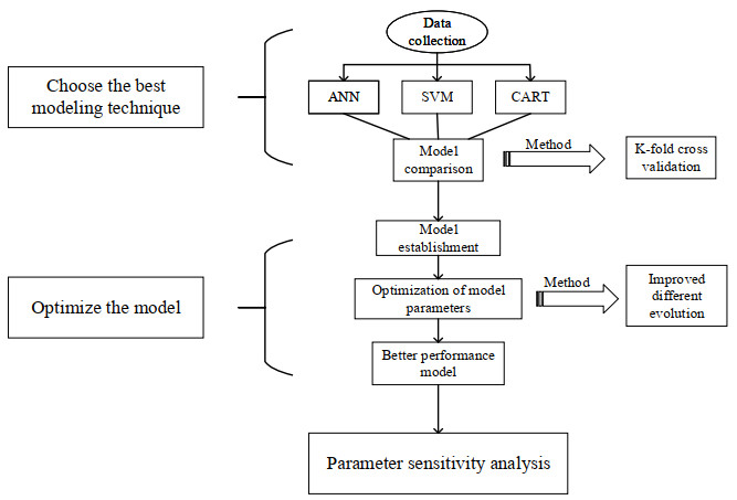
Accurate energy consumption model is the basis of energy saving optimal control of air conditioning system. The existing energy consumption model of air conditioning water system mainly focuses on a certain equipment or a part of the cycle. However, the coupling between water system equipment will affect the setting of optimal energy consumption of equipment. It is necessary to establish the energy consumption model of water system as a whole. However, air conditioning water system is a highly nonlinear complex system, and its precise physical model is difficult to establish. The main goal of this paper is to develop an accurate machine learning modeling and optimization technique to predict the total energy consumption of air conditioning water system by using the actual operation data collected. The main contributions of this work are as follows: (1) Three commonly used machine learning techniques, artificial neural network (ANN), support vector machine (SVM) and classification regression tree (CART), are used to build prediction models of air conditioning water system energy consumption. The results show that all the three models have fast training speed, but the ANN model has better performance in cross-validation. (2) The improved differential evolution algorithm was used to optimize the parameters (initial weights and thresholds) of the ANN, which solved the problem that the ANN is easy to fall into the local optimal solution. The simulation results show that the root mean square error (RMSE) of the improved model decreases by 20.5%, the mean absolute error (MAE) decreases by 30.2%, and the coefficient of determination (R2) increases from 0.9227 to 0.9512. (3) Sensitivity analysis of the established optimization model shows that chilled water flow, chilled water outlet temperature and air conditioning load are the main factors affecting the total energy consumption.

| [1] | EIA, How much energy is consumed in residential and commercial buildings in the United States?, U. S. Energy Inf. Adm. Washington DC, (2014). |
| [2] | L. Yang, Comprehensive Design of Building Energy Conservation, China Building Materials Industry Press, 2014. |
| [3] |
A. M. Georgescu, C. I. Cosoiu, S. Perju, S. C. Georgescu, L. Hasegan, A. Anton, Estimation of the efficiency for variable speed pumps in EPANET compared with experimental data, Procedia Eng., 89 (2014), 1404–1411. https://doi.org/10.1016/j.proeng.2014.11.466 doi: 10.1016/j.proeng.2014.11.466

|
| [4] |
K. Lee, T. Cheng. A simulation-optimization approach for energy efficiency of chilled water system, Energy Build., 54 (2012), 290–296. https://doi.org/10.1016/j.enbuild.2012.06.028 doi: 10.1016/j.enbuild.2012.06.028
|
| [5] |
M. Ali, V. Vukovic, M. Sahir, G. Fontanella, Energy analysis of chilled water system configurations using simulation-based optimization, Energy Build., 59 (2013), 111–122. https://doi.org/10.1016/j.enbuild.2012.12.011 doi: 10.1016/j.enbuild.2012.12.011
|
| [6] |
M. Karami, L. Wang, Particle swarm optimization for control operation of an all-variable speed water-cooled chiller plant, Appl. Therm. Eng., 130 (2018), 962–978. https://doi.org/10.1016/j.applthermaleng.2017.11.037 doi: 10.1016/j.applthermaleng.2017.11.037
|
| [7] | P. Musynski, Impeller pumps: relating η and n, World Pumps, 7 (2010), 25–29. https://doi.org/10.1016/S0262-1762(10)70198-X |
| [8] | Y. D. Ma, M. Maasoumy, Optimal control for the operation of building cooling systems with VAV boxes, Technical report, UC Berkeley, 2011. |
| [9] | H. Meng, W. Long, S. W. Wang, Cooling tower model for system simulation and its experiment validation, HVAC, 34 (2004), 1–5. |
| [10] | EPA, Introduction to indoor air quality, 2018. Available from: https://www.epa.gov/indoor-air-quality-iaq/introduction-indoor-air-quality. |
| [11] |
Y. C. Chang, Sequencing of chillers by estimating chiller power consumption using arterial neural networks, Build. Environ., 42 (2007), 180–188. https://doi.org/10.1016/j.buildenv.2005.08.033. doi: 10.1016/j.buildenv.2005.08.033
|
| [12] |
T. S. Lee, W. C. Lu, An evaluation of empirically-based models for predicting energy performance of vapor-compression water chillers, Appl. Energy, 87 (2010), 3486–3493. https://doi.org/10.1016/j.apenergy.2010.05.005 doi: 10.1016/j.apenergy.2010.05.005
|
| [13] |
X. C. Xi, A. N. Poo, S. K. Chou, Support vector regression model predictive control on a HVAC plant, Control Eng. Pract., 15 (2007), 897–908. https://doi.org/10.1016/j.conengprac.2006.10.010 doi: 10.1016/j.conengprac.2006.10.010
|
| [14] | C. Yang, S. Létourneau, H. Guo, Developing data-driven models to predict BEMS energy consumption for demand response systems, in Modern Adv. Appl. Intell., (2014), 188–197. https://doi.org/10.1007/978-3-319-07455-9_20 |
| [15] |
R. Talib, N. Nabil, W. Choi, Optimization-based data-enabled modeling technique for HVAC systems components, Buildings, 10 (2020), 163. https://doi.org/10.3390/buildings10090163 doi: 10.3390/buildings10090163
|
| [16] |
F. Yan, Z. B. Lin, X. Y. Wang, F. Azarmi, K. Sobolev, Evaluation and prediction of bond strength of GFRP-bar reinforced concrete using artificial neural network optimized with genetic algorithm, Compos. Struct., 161 (2017), 441–452. https://doi.org/10.1016/j.compstruct.2016.11.068 doi: 10.1016/j.compstruct.2016.11.068
|
| [17] |
M. R. Chen, B. P. Chen, G. Q. Zeng, K. D. Lu, P. Chu, An adaptive fractional-order BP neural network based on extremal optimization for handwritten digits recognition, Neurocomputing, 391 (2020), 260–272. https://doi.org/10.1016/j.neucom.2018.10.090 doi: 10.1016/j.neucom.2018.10.090
|
| [18] |
J. Wu, Y. M. Cheng, C. Liu, I. Lee, W. Huang, A BP neural network based on GA for optimizing energy consumption of copper electrowinning, Math. Prob. Eng., 2020 (2020), 1026128. https://doi.org/10.1155/2020/1026128 doi: 10.1155/2020/1026128
|
| [19] |
J. F. Huang, L. L. He. Application of improved PSO-BP neural network in customer churn warning, Proc. Comput. Sci., 131 (2018), 1238–1246. https://doi.org/10.1016/j.procs.2018.04.336 doi: 10.1016/j.procs.2018.04.336
|
| [20] |
Y. Deng, H. J. Xiao, J. X. Xu, H. Wang, Prediction model of PSO-BP neural network on coliform amount in special food, Saudi J. Biol. Sci., 26 (2019), 1154–1160. https://doi.org/10.1016/j.sjbs.2019.06.016 doi: 10.1016/j.sjbs.2019.06.016
|
| [21] |
H. R. Tian, P. X. Wang, K. Tansey, S. Zhang, J. Zhang, H. Li, An IPSO-BP neural network for estimating wheat yield using two remotely sensed variables in the Guanzhong Plain, PR China, Comput. Electron. Agric., 169 (2019). https://doi.org/10.1016/j.compag.2019.105180 doi: 10.1016/j.compag.2019.105180
|
| [22] |
W. Q. Jing, J. Q. Yu, L. Wei, C. Li, X. Liu, Energy-saving diagnosis model of central air-conditioning refrigeration system in large shopping mall, Energy Rep., 7 (2021), 4035–4046. https://doi.org/10.1016/j.egyr.2021.06.083 doi: 10.1016/j.egyr.2021.06.083
|
| [23] |
R. Storn, K. Price, Differential Evolution: A simple and efficient adaptive scheme for global optimization over continuous spaces, J. Global Optim., 11 (1997), 341–359. https://doi.org/10.1023/A:1008202821328 doi: 10.1023/A:1008202821328
|
| [24] | W. X. Ji, Z. H. Chen, Z. Fang, Air conditioning load prediction based on DE-BP algorithm, Sichuan Build. Sci., 36 (2010), 268–270. |
| [25] | F. Cai, Application research on optimal operation of air conditioning water system, Master Thesis, University of Science and Technology Liaoning, China, 2018. |
| [26] |
H. Huerto-Cardenas, F. Leonforte, N. Aste, C. Del Pero, G. Evola, V. Costanzo, et al., Validation of dynamic hygrothermal simulation models for historical buildings: State of the art, research challenges and recommendations, Build. Environ., 180 (2020). https://doi.org/10.1016/j.buildenv.2020.107081 doi: 10.1016/j.buildenv.2020.107081
|
| [27] | ASHRAE Guideline 14-2014, Measurement of Energy, Demand, and Water Savings, Atlanta, USA, 2014. |
| [28] |
J. Zhang, A. C. Sanderson. Jade: adaptive differential evolution with optional external archive. IEEE Trans. Evol. Comput., 13 (2009), 945–958. https://doi.org/10.1109/TEVC.2009.2014613 doi: 10.1109/TEVC.2009.2014613
|


Figures(8) / Tables(3)

Qixin Zhu, Mengyuan Liu, Hongli Liu, Yonghong Zhu. Application of machine learning and its improvement technology in modeling of total energy consumption of air conditioning water system[J]. Mathematical Biosciences and Engineering, 2022, 19(5): 4841-4855. doi: 10.3934/mbe.2022226


 DownLoad: