Camera devices are being deployed everywhere. Cities, enterprises, and more and more smart homes are using camera devices. Fine-grained identification of devices brings an in-depth understanding of the characteristics of these devices. Identifying the device type helps secure the device safe. But, existing device identification methods have difficulty in distinguishing fine-grained types of devices. To address this challenge, we propose a fine-grained identification method based on the camera deviceso inherent features. First, feature selection is based on the coverage and differences of the inherent features type. Second, the features are classified according to their representation. A design feature similarity calculation strategy (FSCS) for each type of feature is established. Then the feature weights are determined based on feature entropy. Finally, we present a device similarity model based on the FSCS and feature weights. And we use this model to identify the fine-grained type of a target device. We have evaluated our method on Dahua and Hikvision camera devices. The experimental results show that we can identify the deviceos fine-grained type when some inherent feature values are missing. Even when the inherent feature pmissing rateq is 50%, the average accuracy still exceeds 80%.
Citation: Ruimin Wang, Ruixiang Li, Weiyu Dong, Zhiyong Zhang, Liehui Jiang. Fine-grained identification of camera devices based on inherent features[J]. Mathematical Biosciences and Engineering, 2022, 19(4): 3767-3786. doi: 10.3934/mbe.2022173
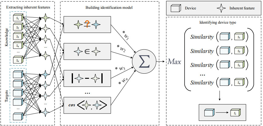
Camera devices are being deployed everywhere. Cities, enterprises, and more and more smart homes are using camera devices. Fine-grained identification of devices brings an in-depth understanding of the characteristics of these devices. Identifying the device type helps secure the device safe. But, existing device identification methods have difficulty in distinguishing fine-grained types of devices. To address this challenge, we propose a fine-grained identification method based on the camera deviceso inherent features. First, feature selection is based on the coverage and differences of the inherent features type. Second, the features are classified according to their representation. A design feature similarity calculation strategy (FSCS) for each type of feature is established. Then the feature weights are determined based on feature entropy. Finally, we present a device similarity model based on the FSCS and feature weights. And we use this model to identify the fine-grained type of a target device. We have evaluated our method on Dahua and Hikvision camera devices. The experimental results show that we can identify the deviceos fine-grained type when some inherent feature values are missing. Even when the inherent feature pmissing rateq is 50%, the average accuracy still exceeds 80%.

| [1] |
R. Li, R. Xu, Y. Ma, X. Luo, LandmarkMiner: Street-level network landmarks mining method for IP geolocation, ACM Trans. Internet Things, 2 (2021), 1–22. https://doi.org/10.1145/3457409 doi: 10.1145/3457409

|
| [2] |
V. F. Taylor, R. Spolaor, M. Conti, I. Martinovic, Robust smartphone app identification via encrypted network traffic analysis, IEEE Trans. Inf. Forensics Secur., 13 (2017), 63–78. https://doi.org/10.1109/TIFS.2017.2737970 doi: 10.1109/TIFS.2017.2737970
|
| [3] |
N. G. B. Amma, S. Selvakumar, R. L. Velusamy, A statistical approach for detection of denial of service attacks in computer networks, IEEE Trans. Network Service Manage., 17 (2020), 2511–2522. https://doi.org/10.1109/TNSM.2020.3022799 doi: 10.1109/TNSM.2020.3022799
|
| [4] | D. Goldman, Shodan: The scariest search engine on the Internet, 2013. Available from: https://money.cnn.com/2013/04/08/technology/security/shodan/. |
| [5] | G. F. Lyon, Nmap Network Scanning: The Official Nmap Project Guide to Network Discovery and Security Scanning, Nmap Project, (2009), 5–12. |
| [6] | Z. Durumeric, E. Wustrow, J. A. Halderman, ZMap: Fast Internet-wide scanning and its security applications, USENIX Secur. Symp., (2013), 605–620. https://dl.acm.org/doi/10.5555/2534766.2534818 |
| [7] | Z. Durumeric, D. Adrian, A. Mirian, M. Bailey, J. A. Halderman, A search engine backed by internet-wide scanning, in Proceedings of the 22nd ACM SIGSAC Conference on Computer and Communications Security, (2015), 542–553. https://doi.org/10.1145/2810103.2813703 |
| [8] | R. Li, M. Shen, H. Yu, C. Li, P. Duan, L. Zhu, A survey on cyberspace search engines, in China Cyber Security Annual Conference, Springer, Singapore, (2020), 206–214. https://doi.org/10.1007/978-981-33-4922-3_15 |
| [9] | Y. Meidan, M. Bohadana, A. Shabtai, J. Guarnizo, ProfilIoT: A machine learning approach for IoT device identification based on network traffic analysis, in Proceedings of the 32nd ACM Symposium on Applied Computing, (2017), 506–509. https://doi.org/10.1145/3019612.3019878 |
| [10] | M. Miettinen, S. Marchal, I. Hafeez, N. Asokan, A. Sadeghi, S. Tarkoma, Iot sentinel: Automated device-type identification for security enforcement in iot, in 2017 IEEE 37th International Conference on Distributed Computing Systems (ICDCS), (2017), 2511–2514. https://doi.org/10.1109/ICDCS.2017.284 |
| [11] | A. Sivanathan, D. Sherratt, H. H. Gharakheili, A. Radford, C. Wijenayake, A. Vishwanath, et al., Characterizing and classifying IoT traffic in smart cities and campuses, in 2017 IEEE Conference on Computer Communications Workshops (INFOCOM WKSHPS), (2017), 559–564. https://doi.org/10.1109/INFCOMW.2017.8116438 |
| [12] | W. Cheng, Z. Ding, C. Xu, X. Wu, Y. Xia, J. Mao, RAFM: A real-time auto detecting and fingerprinting method for IoT devices, in Journal of Physics: Conference Series, 1518 (2020), 12043–12050. https://dx.doi.org/10.1088/1742-6596/1518/1/012043 |
| [13] |
D. E. Rumelhart, G. E. Hinton, R. J. Williams, Learning representations by back propagating errors, Nature, 323 (1986), 533–536. https://doi.org/10.1038/323533a0 doi: 10.1038/323533a0
|
| [14] |
C. Cortes, V. Vapnik, Support-vector networks, Mach. Learn., 20 (1995), 273–297. https://doi.org/10.1023/A:1022627411411 doi: 10.1023/A:1022627411411
|
| [15] |
T. Hastie, R. Tibshirani, Discriminant adaptive nearest neighbor classification, IEEE Trans. Pattern Anal. Mach. Intell., 18 (1996), 607–616. https://doi.org/10.1109/34.506411 doi: 10.1109/34.506411
|
| [16] |
K. Yang, Q. Li, L. Sun, Towards automatic fingerprinting of IoT devices in the cyberspace, Comput. Networks, 148 (2019), 318–327. https://doi.org/10.1016/j.comnet.2018.11.013 doi: 10.1016/j.comnet.2018.11.013
|
| [17] |
A. Sivanathan, H. H. Gharakheili, F. Loi, A. Radford, C. Wijenayake, A. Vishwanath, et al., Classifying IoT devices in smart environments using network traffic characteristics, IEEE Trans. Mobile Comput., 18 (2019), 1745–1759. https://doi.org/10.1109/TMC.2018.2866249 doi: 10.1109/TMC.2018.2866249
|
| [18] |
S. V. Radhakrishnan, A. S. Uluagac, R. Beyah, GTID: A technique for physical device and device type fingerprinting, IEEE Trans. Dependable Secure Comput., 12 (2015), 519–532. https://doi.org/10.1109/TDSC.2014.2369033 doi: 10.1109/TDSC.2014.2369033
|
| [19] |
Y. Zou, S. Liu, N. Yu, H. Zhu, L. Sun, H. Li, et al., IoT device recognition framework based on web search, J. Cyber Secur., 3 (2018), 25–40. https://doi.org/10.19363/J.cnki.cn10-1380/tn.2018.07.03 doi: 10.19363/J.cnki.cn10-1380/tn.2018.07.03
|
| [20] | X. Feng, Q. Li, H. Wang, L. Sun, Acquisitional rule-based engine for discovering internet-of-things devices, in Proceedings of the 27th USENIX Security Symposium, 148 (2018), 327–341. https://dl.acm.org/doi/10.5555/3277203.3277228 |
| [21] |
S. Agarwal, P. Oser, S. Lueders, Detecting IoT devices and how they put large heterogeneous networks at security risk, Sensor, 19 (2019), 4107–4107. https://doi.org/10.3390/s19194107 doi: 10.3390/s19194107
|
| [22] |
T. Kohno, A. Broido, K. C. Claffy, Remote physical device fingerprinting, IEEE Trans. Dependable Secure Comput., 2 (2005), 93–108. https://doi.org/10.1109/TDSC.2005.26 doi: 10.1109/TDSC.2005.26
|
| [23] | S. J. Murdoch, Hot or not: Revealing hidden services by their clock skew, in Proceedings of the 13th ACM Conference on Computer and Communications Security, (2006), 27–36. https://doi.org/10.1145/1180405.1180410 |
| [24] | S. Zander, S. J. Murdoch, An improved clock-skew measurement technique for revealing hidden services, in Proceedings of the 17th USENIX Security Symposium, (2008), 211–225. https://dl.acm.org/doi/10.5555/1496711.1496726 |
| [25] | D. J. Huang, K. T. Yang, C. C. Ni, W. C. Teng, T. R. Hsiang, Y. J. Lee, Clock skew based client device identification in cloud environments, in Proceedings of the 26th IEEE International Conference on Advanced Information Networking and Applications, (2012), 526–533. https://doi.org/10.1109/AINA.2012.51 |
| [26] | Y. Vanaubel, J. J. Pansiot, P. Merindol, B. Donnet, Network fingerprinting: TTL-based router signatures, in Proceedings of the 2013 Conference on Internet Measurement Conference, (2013), 369–376. https://doi.org/10.1145/2504730.2504761 |
| [27] |
T. Kohno, A. Broido, K. C. Claffy, Remote physical device fingerprinting, IEEE Trans. Dependable Secure Comput., 2 (2005), 93–108. https://doi.org/10.1109/SP.2005.18 doi: 10.1109/SP.2005.18
|


Figures(5) / Tables(3)

Ruimin Wang, Ruixiang Li, Weiyu Dong, Zhiyong Zhang, Liehui Jiang. Fine-grained identification of camera devices based on inherent features[J]. Mathematical Biosciences and Engineering, 2022, 19(4): 3767-3786. doi: 10.3934/mbe.2022173


 DownLoad: