We propose and study computationally a novel non-local multiscale moving boundary mathematical model for tumour and oncolytic virus (OV) interactions when we consider the go or grow hypothesis for cancer dynamics. This spatio-temporal model focuses on two cancer cell phenotypes that can be infected with the OV or remain uninfected, and which can either move in response to the extracellular-matrix (ECM) density or proliferate. The interactions between cancer cells, those among cancer cells and ECM, and those among cells and OV occur at the macroscale. At the micro-scale, we focus on the interactions between cells and matrix degrading enzymes (MDEs) that impact the movement of tumour boundary. With the help of this multiscale model we explore the impact on tumour invasion patterns of two different assumptions that we consider in regard to cell-cell and cell-matrix interactions. In particular we investigate model dynamics when we assume that cancer cell fluxes are the result of local advection in response to the density of extracellular matrix (ECM), or of non-local advection in response to cell-ECM adhesion. We also investigate the role of the transition rates between mainly-moving and mainly-growing cancer cell sub-populations, as well as the role of virus infection rate and virus replication rate on the overall tumour dynamics.
Citation: Abdulhamed Alsisi, Raluca Eftimie, Dumitru Trucu. Non-local multiscale approach for the impact of go or grow hypothesis on tumour-viruses interactions[J]. Mathematical Biosciences and Engineering, 2021, 18(5): 5252-5284. doi: 10.3934/mbe.2021267
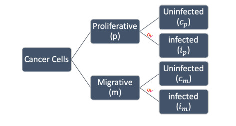
We propose and study computationally a novel non-local multiscale moving boundary mathematical model for tumour and oncolytic virus (OV) interactions when we consider the go or grow hypothesis for cancer dynamics. This spatio-temporal model focuses on two cancer cell phenotypes that can be infected with the OV or remain uninfected, and which can either move in response to the extracellular-matrix (ECM) density or proliferate. The interactions between cancer cells, those among cancer cells and ECM, and those among cells and OV occur at the macroscale. At the micro-scale, we focus on the interactions between cells and matrix degrading enzymes (MDEs) that impact the movement of tumour boundary. With the help of this multiscale model we explore the impact on tumour invasion patterns of two different assumptions that we consider in regard to cell-cell and cell-matrix interactions. In particular we investigate model dynamics when we assume that cancer cell fluxes are the result of local advection in response to the density of extracellular matrix (ECM), or of non-local advection in response to cell-ECM adhesion. We also investigate the role of the transition rates between mainly-moving and mainly-growing cancer cell sub-populations, as well as the role of virus infection rate and virus replication rate on the overall tumour dynamics.

| [1] |
A. Corcoran, R, F. Del Maestro, Testing the "go or grow" hypothesis in human medulloblastoma cell lines in two and three dimensions, Neurosurgery, 53 (2003), 174-185. doi: 10.1227/01.NEU.0000072442.26349.14

|
| [2] |
A. Giese, M. A. Loo, N. Tran, D. Haskett, S. W. Coons, M. E. Berens, Dichotomy of astrocytoma migration and proliferation, Int. J. Cancer, 67 (1996), 275-282. doi: 10.1002/(SICI)1097-0215(19960717)67:2<275::AID-IJC20>3.0.CO;2-9
|
| [3] |
A. Giese, R. Bjerkvig, M. E. Berens, M. Westphal, Cost of migration: invasion of malignant gliomas and implications for treatment, J. Clin. Oncol., 21 (2003), 1624-1636. doi: 10.1200/JCO.2003.05.063
|
| [4] |
K. S. Hoek, O. M. Eichhoff, N. C. Schlegel, U. Dobbeling, N. Kobert, L. Schaerer, et al., In vivo switching of human melanoma cells between proliferative and invasive states, Cancer Res., 68 (2008), 650-656. doi: 10.1158/0008-5472.CAN-07-2491
|
| [5] |
J. Godlewski, M. O. Nowicki, A. Bronisz, G. Nuovo, J. Palatini, M. D. Lay, et al., MicroRNA-451 regulates LKB1/AMPK signaling and allows adaptation to metabolic stress in glioma cells, Mol. Cell, 37 (2010), 620-632. doi: 10.1016/j.molcel.2010.02.018
|
| [6] |
L. Jerby, L. Wolf, C. Denkert, G. Y. Stein, M. Hilvo, M. Oresic, et al., Metabolic associations of reduced proliferation and oxidative stress in advanced breast cancer, Cancer Res., 72 (2012), 5712-5720. doi: 10.1158/0008-5472.CAN-12-2215
|
| [7] | J. Metzcar, Y. Wang, R. Heiland, P. Macklin, A review of cell-based computational modeling in cancer biology, JCO Clin. Cancer Inf., (2019), 1-13. |
| [8] | J. A. Gallaher, J. S. Brown, A. R. A. Anderson, The impact of proliferation-migration tradeoffs on phenotypic evolution in cancer, Sci. Rep., 9 (2019), 1-10. |
| [9] |
M. Tektonidis, H. Hatzikirou, A. Chauvière, M. Simon, K. Schaller, A. Deutsch, Identification of intrinsic in vitro cellular mechanisms for glioma invasion, J. Theor. Biol., 287 (2011), 131-147. doi: 10.1016/j.jtbi.2011.07.012
|
| [10] |
T. Garay, É. Juhász, E. Molnár, M. Eisenbauer, A. Czirók, B. Dekan, et al., Cell migration or cytokinesis and proliferation? - Revisiting the "go or grow" hypothesis in cancer cells in vitro, Exp. Cell Res., 319 (2013), 3094-3103. doi: 10.1016/j.yexcr.2013.08.018
|
| [11] |
S. T. Vittadello, S. W. McCue, G. Gunasingh, N. K. Haass, M. J. Simpson, Examining go-or-grow using fluorescent cell-cycle indicators and cell-cycle-inhibiting drugs, Biophys. J., 118 (2020), 1243-1247. doi: 10.1016/j.bpj.2020.01.036
|
| [12] |
J. C. L. Alfonso, K. Talkenberger, M. Seifert, B. Klink, A. Hawkins-Daarud, K. R. Swanson, et al., The biology and mathematical modelling of glioma invasion: a review, J. R. Soc. Interface, 14 (2017), 20170490. doi: 10.1098/rsif.2017.0490
|
| [13] | K. Böttger, H. Hatzikirou, A. Chauviere, A. Deutsch, Investigation of the migration/proliferation dichotomy and its impact on avascular glioma invasion, Math. Model. Nat. Phenom., 7 (2012), 105-135. |
| [14] |
K. Böttger, H. Hatzikirou, A. Voss-Böhme, E. A. Cavalcanti-Adam, M. A. Herrero, A. Deutsch, An emerging Allee effect is critical for tumor initiation and persistence, PLOS Comput. Biol., 11 (2015), e1004366. doi: 10.1371/journal.pcbi.1004366
|
| [15] | P. Gerlee, S. Nelander, The impact of phenotypic switching on glioblastoma growth and invasion, PLoS Comput. Biol., 8 (2012). |
| [16] |
H. Hatzikirou, D. Basanta, M. Simon, K. Schaller, A. Deutsch, 'Go or Grow': the key to the emergence of invasion in tumour progression?, Math. Med. Biol., 29 (2012), 49-65. doi: 10.1093/imammb/dqq011
|
| [17] | H. N. Weerasinghe, P. M. Burrage, K. Burrage, D. V. Nicolau, Mathematical models of cancer cell plasticity, J. Oncol., (2019), 1-C. |
| [18] | Y. Kim, H. Kang, S. Lawler, The role of the miR-451-AMPK signaling pathway in regulation of cell migration and proliferation in glioblastoma, in Mathematical Models of Tumor-Immune System Dynamics, Springer, New York, (2014), 25-155. |
| [19] |
A. V. Kolobov, V. V. Gubernov, A. A. Polezhaev, Autowaves in the model of infiltrative tumour growth with migration-proliferation dichotomy, Math. Model. Nat. Phenom., 6 (2011), 27-38. doi: 10.1051/mmnp/20116703
|
| [20] |
K. Pham, A. Chauviere, H. Hatzikirou, X. Li, H. M. Byrne, V. Cristini, et al., Density-dependent quiescence in glioma invasion: instability in a simple reaction-diffusion model for the migration/proliferation dichotomy, J. Biol. Dyn., 6 (2012), 54-71. doi: 10.1080/17513758.2011.590610
|
| [21] |
O. Saut, J. B. Lagaert, T. Colin, H. M. Fathallah-Shaykh, A multilayer grow-or-go model for GBM: effects of invasive cells and anti-angiogenesis on growth, Bull. Math. Biol., 76 (2014), 2306-2333. doi: 10.1007/s11538-014-0007-y
|
| [22] |
T. L. Stepien, E. M. Rutter, Y. Kuang, Traveling waves of a go-or-grow model of glioma growth, SIAM J. Appl. Math., 78 (2018), 1778-1801. doi: 10.1137/17M1146257
|
| [23] |
C. Stinner, C. Surulescu, A. Uatay, Global existence for a go-or-grow multiscale model for tumor invasion with therapy, Math. Model. Methods Appl. Sci., 26 (2016), 2163-2201. doi: 10.1142/S021820251640011X
|
| [24] |
E. Scribner, O. Saut, P. Province, A. Bag, T. Colin, H. M. Fathallah-Shaykh, Effects of anti-angiogenesis on glioblastoma growth and migration: model to clinical predictions, PLoS One, 9 (2014), e115018. doi: 10.1371/journal.pone.0115018
|
| [25] | A. Zhigun, C. Surulescu, A. Hunt, A strongly degenerate diffusion-haptotaxis model of tumour invasion under the go-or-grow dichotomy hypothesis, Math. Methods Appl. Sci., 41 (2018), 2403-2428. |
| [26] | M. A. Lewis, G. Schmitz, Biological invasion of an organism with separate mobile and stationary states: Modeling and analysis, Forma, 11 (1996), 1-25. |
| [27] | X. Ma, M. E. Schickel, M. D. Stevenson, A. L. Sarang-Sieminski, K. J. Gooch, S. N. Ghadiali, et al., Fibres in the extracellular matrix enable long-range stress transmission between cells, Biophys. J., 104 (2013), 1410-1418. |
| [28] |
N. J. Armstrong, K. J. Painter, J. A. Sherratt, A continuum approach to modelling cell-cell adhesion, J. Theor. Biol., 243 (2006), 98-113. doi: 10.1016/j.jtbi.2006.05.030
|
| [29] |
T. Alzahrani, R. Eftimie, D. Trucu, Multiscale modelling of cancer response to oncolytic viral therapy, Math. Biosci., 310 (2019), 76-95. doi: 10.1016/j.mbs.2018.12.018
|
| [30] | J. Ahn, M. Chae, J. Lee, Nonlocal adhesion models for two cancer cell phenotypes in a multidimensional bounded domain, Z. Angew. Math. Phys., 72 (2021), 1-28. |
| [31] | M. Eckardt, K. J. Painter, C. Surulescu, A. Zhigun, Nonlocal and local models for taxis in cell migration: a rigorous limit procedure, J. Math. Biol., 81 (2020), 1251-1298. |
| [32] |
R. Alemany, Viruses in cancer treatment, Clin. Transl. Oncol., 15 (2013), 182-188. doi: 10.1007/s12094-012-0951-7
|
| [33] |
M. Vähä-Koskela, A. Hinkkanen, Tumor restrictions to oncolytic virus, Biomedicines, 2 (2014), 163-194. doi: 10.3390/biomedicines2020163
|
| [34] | A. Alsisi, R. Eftimie, D. Trucu, Non-local multiscale approaches for tumour-oncolytic viruses interactions, Math. Appl. Sci. Eng., 99 (2020), 1-27. |
| [35] |
D. Trucu, P. Lin, M. A. J. Chaplain, Y. Wang, A multiscale moving boundary model Arising in cancer invasion, Multiscale Model. Simul., 11 (2013), 309-335. doi: 10.1137/110839011
|
| [36] |
N. Bhagavathula, A. W. Hanosh, K. C. Nerusu, H. Appelman, S. Chakrabarty, J. Varani, Regulation of E-cadherin and $\beta$-catenin by Ca2+ in colon carcinoma is dependent on calcium-sensing receptor expression and function, Int. J. Cancer, 121 (2007), 1455-1462. doi: 10.1002/ijc.22858
|
| [37] |
U. Cavallaro, G. Christofori, Cell adhesion in tumor invasion and metastasis: loss of the glue is not enough, Biochim. Biophys. Acta Rev. Cancer, 1552 (2001), 39-45. doi: 10.1016/S0304-419X(01)00038-5
|
| [38] |
J. D. Humphries, Integrin ligands at a glance, J. Cell Sci., 119 (2006), 3901-3903. doi: 10.1242/jcs.03098
|
| [39] |
K. S. Ko, P. D. Arora, V. Bhide, A. Chen, C. A. McCulloch, Cell-cell adhesion in human fibroblasts requires calcium signaling, J. Cell Sci., 114 (2001), 1155-1167. doi: 10.1242/jcs.114.6.1155
|
| [40] | B. P. L. Wijnhoven, W. N. M. Dinjens, M. Pignatelli, E-cadherin-catenin cell-cell adhesion complex and human cancer, Br. J. Surg., 87 (2000), 992-1005. |
| [41] |
M. A. J. Chaplain, G. Lolas, Mathematical modelling of cancer invasion of tissue: dynamic heterogeneity, Networks Heterog. Media, 1 (2006), 399-439. doi: 10.3934/nhm.2006.1.399
|
| [42] | M. J. Oudin, O. Jonas, T. Kosciuk, L. C. Broye, B. C. Guido, J. Wyckoff, et al., Tumor cell-driven extracellular matrix remodeling drives haptotaxis during metastatic progression, Cancer Discovery, 6 (2016), 516-531. |
| [43] |
P. Domschke, D. Trucu, A. Gerisch, M. A. J. Chaplain, Mathematical modelling of cancer invasion: Implications of cell adhesion variability for tumour infiltrative growth patterns, J. Theor. Biol., 361 (2014), 41-60. doi: 10.1016/j.jtbi.2014.07.010
|
| [44] |
A. Gerisch, M. A. J. Chaplain, Mathematical modelling of cancer cell invasion of tissue: Local and non-local models and the effect of adhesion, J. Theor. Biol., 250 (2008), 684-704. doi: 10.1016/j.jtbi.2007.10.026
|
| [45] |
Z. Gu, F. Liu, E. A. Tonkova, S. Y. Lee, D. J. Tschumperlin, M. B. Brenner, Soft matrix is a natural stimulator for cellular invasiveness, Mol. Biol. Cell, 25 (2014), 457-469. doi: 10.1091/mbc.e13-05-0260
|
| [46] |
A. M. Hofer, S. Curci, M. A. Doble, E. M. Brown, D. I. Soybel, Intercellular communication mediated by the extracellular calcium-sensing receptor, Nat. Cell Biol., 2 (2000), 392-398. doi: 10.1038/35017020
|
| [47] |
R. Shuttleworth, D. Trucu, Multiscale modelling of fibres dynamics and cell adhesion within moving boundary cancer invasion, Bull. Math. Biol., 81 (2019), 2176-2219. doi: 10.1007/s11538-019-00598-w
|
| [48] | C. Guiot, P. Degiorgis, P. Delsanto, P. Gabriele, T. Diesboeck, Does tumour growth follow a "universal law"?, J. Theor. Biol., 225 (2003), 147-151. |
| [49] | A. Laird, Dynamics of tumour growth, Br. J. Cancer, 18 (1964), 490-502. |
| [50] |
D. Hanahan, R. A. Weinberg, Hallmarks of cancer: The next generation, Cell, 144 (2011), 646-674. doi: 10.1016/j.cell.2011.02.013
|
| [51] | R. A. Weinberg, The Biology of Cancer, Garland Science, New York, 2006. |
| [52] | P. R. Halmos, Measure Theory, Springer-Verlag, New York, USA, 1974. |
| [53] | S. Suveges, R. Eftimie, D. Trucu, Directionality of macrophages movement in tumour invasion: A multiscale moving-boundary approach, Bull. Math. Biol., 82 (2020), 1-48. |
| [54] |
B. I. Camara, H. Mokrani, E. Afenya, Mathematical modeling of glioma therapy using oncolytic viruses, Math. Biosci. Eng., 10 (2013), 565-578. doi: 10.3934/mbe.2013.10.565
|
| [55] |
K. J. Painter, N. J. Armstrong, J. A. Sherratt, The impact of adhesion on cellular invasion processes in cancer and development, J. Theor. Biol., 264 (2010), 1057-1067. doi: 10.1016/j.jtbi.2010.03.033
|
| [56] |
R. Shuttleworth, D. Trucu, Multiscale dynamics of a heterotypic cancer cell population within a fibrous extracellular matrix, J. Theor. Biol., 486 (2020), 110040. doi: 10.1016/j.jtbi.2019.110040
|
| [57] |
L. Peng, D. Trucu, P. Lin, A. Thompson, M. A. J. Chaplain, A multiscale mathematical model of tumour invasive growth, Bull. Math. Biol., 79 (2017), 389-429. doi: 10.1007/s11538-016-0237-2
|
| [58] |
T. Alzahrani, R. Eftimie, D. Trucu, Multiscale moving boundary modelling of cancer interactions with a fusogenic oncolytic virus: The impact of syncytia dynamics, Math. Biosci., 323 (2020), 108296. doi: 10.1016/j.mbs.2019.108296
|


Figures(9) / Tables(1)

Abdulhamed Alsisi, Raluca Eftimie, Dumitru Trucu. Non-local multiscale approach for the impact of go or grow hypothesis on tumour-viruses interactions[J]. Mathematical Biosciences and Engineering, 2021, 18(5): 5252-5284. doi: 10.3934/mbe.2021267


 DownLoad: