Control and optimization mechanism of an electromagnetic transducer model with nonlinear magnetic coupling

Hany Bauomy; Hany Bauomy

doi:10.3934/math.2025135

AIMS Mathematics

2025, Volume 10, Issue 2: 2891-2929. doi: 10.3934/math.2025135

Previous Article Next Article

Research article Special Issues

Control and optimization mechanism of an electromagnetic transducer model with nonlinear magnetic coupling

Hany Bauomy ^,

Department of Mathematics, College of Science and Humanities in Alkharj, Prince Sattam Bin Abdulaziz University, Alkharj 11942, Saudi Arabia

Received: 28 November 2024 Revised: 02 January 2025 Accepted: 08 February 2025 Published: 17 February 2025
MSC : 34A34, 37N35, 70J99, 70K20, 74H10

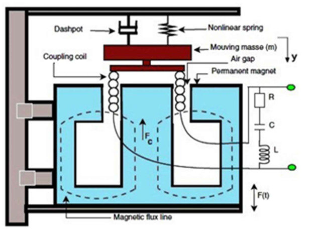
This paper presents a novel nonlinear proportional-derivative cubic velocity feedback (NPDVF) controller for controlling vibrations in systems with both mechanical and electrical components subjected to mixed forces. The proposed controller aims to address the challenges posed by nonlinear bifurcations, unstable motion, and vibrations. The effectiveness of the controller demonstrated through numerical simulations, where it shown to significantly reduce harmful vibrations and stabilize the system under varying operating conditions. To analyze the system, a perturbation technique employed to derive approximate solutions to the system's equations up to the second order at simultaneous resonance case ($ {\varOmega }_{2}\cong {\omega }_{1}, {\varOmega }_{4}\cong {\omega }_{2} $). A comparative analysis with other control strategies, such as proportional-derivative (PD) control, sliding mode control (SMC), and model predictive control (MPC), the superior robustness, computational efficiency, and control signal amplitude of the NPDVF controller. Results indicate that the proposed approach not only outperforms traditional methods in terms of energy efficiency and computational cost but also maintains robust performance even in the presence of nonlinearities and parameter uncertainties. The findings support the potential application of the NPDVF controller in real-time vibration control systems.
- mixed excitations,
- electromagnetic transducer,
- perturbation,
- stability,
- NPDCVF controllers
Citation: Hany Bauomy. Control and optimization mechanism of an electromagnetic transducer model with nonlinear magnetic coupling[J]. AIMS Mathematics, 2025, 10(2): 2891-2929. doi: 10.3934/math.2025135

Related Papers:

Abstract

This paper presents a novel nonlinear proportional-derivative cubic velocity feedback (NPDVF) controller for controlling vibrations in systems with both mechanical and electrical components subjected to mixed forces. The proposed controller aims to address the challenges posed by nonlinear bifurcations, unstable motion, and vibrations. The effectiveness of the controller demonstrated through numerical simulations, where it shown to significantly reduce harmful vibrations and stabilize the system under varying operating conditions. To analyze the system, a perturbation technique employed to derive approximate solutions to the system's equations up to the second order at simultaneous resonance case ($ {\varOmega }_{2}\cong {\omega }_{1}, {\varOmega }_{4}\cong {\omega }_{2} $). A comparative analysis with other control strategies, such as proportional-derivative (PD) control, sliding mode control (SMC), and model predictive control (MPC), the superior robustness, computational efficiency, and control signal amplitude of the NPDVF controller. Results indicate that the proposed approach not only outperforms traditional methods in terms of energy efficiency and computational cost but also maintains robust performance even in the presence of nonlinearities and parameter uncertainties. The findings support the potential application of the NPDVF controller in real-time vibration control systems.

References

[1]	R. Yamapi, J. B. C. Orou, P. Woafo, Harmonic oscillations, stability and chaos control in a nonlinear electromechanical system, J. Sound Vib., 259 (2003), 1253–1264. https://doi.org/10.1006/jsvi.2002.5289 doi: 10.1006/jsvi.2002.5289
[2]	Z. M. Ge, T. N. Lin, Chaos, Chaos control and synchronization of electro-mechanical gyrostat system, J. Sound Vib., 259 (2003), 585–603. https://doi.org/10.1006/jsvi.2002.5110 doi: 10.1006/jsvi.2002.5110
[3]	R. Yamapi, S. Bowong, Dynamics and chaos control of the self-sustained electromechanical device with and without discontinuity, Commun. Nonlinear Sci., 11 (2006), 355–375. https://doi.org/10.1016/j.cnsns.2004.09.002 doi: 10.1016/j.cnsns.2004.09.002
[4]	M. Siewe Siewe, F. M. M. Kakmeni, S. Bowong, C. Tchawoua, Non-linear response of a self-sustained electromechanical seismographs to fifth resonance excitations and chaos control, Chaos Soliton. Fract., 29 (2006), 431–445. https://doi.org/10.1016/j.chaos.2005.08.210 doi: 10.1016/j.chaos.2005.08.210
[5]	R. Yamapi, F. M. M. Kakmeni, J. B. C. Orou, Nonlinear dynamics and synchronization of coupled electromechanical systems with multiple functions, Commun. Nonlinear Sci., 12 (2007), 543–567. https://doi.org/10.1016/j.cnsns.2005.05.003 doi: 10.1016/j.cnsns.2005.05.003
[6]	R. Yamapi, M. A. Aziz-Alaoui, Vibration analysis and bifurcations in the self-sustained electromechanical system with multiple functions, Commun. Nonlinear Sci., 12 (2007), 1534–1549. https://doi.org/10.1016/j.cnsns.2006.03.001 doi: 10.1016/j.cnsns.2006.03.001
[7]	C. A. K. Kwuimy, P. Woafo, Dynamics of a self-sustained electromechanical system with flexible arm and cubic coupling, Commun. Nonlinear Sci., 12 (2007), 1504–1517. https://doi.org/10.1016/j.cnsns.2006.03.003 doi: 10.1016/j.cnsns.2006.03.003
[8]	C. A. K. Kwuimy, P. Woafo, Dynamics, chaos and synchronization of self-sustained electromechanical systems with clamped-free flexible arm, Nonlinear Dyn., 53 (2008), 201–213. https://doi.org/10.1007/s11071-007-9308-0 doi: 10.1007/s11071-007-9308-0
[9]	G. S. M. Ngueuteu, R. Yamapi, P. Woafo, Effects of higher nonlinearity on the dynamics and synchronization of two coupled electromechanical devices, Commun. Nonlinear Sci., 13 (2008), 1213–1240. https://doi.org/10.1016/j.cnsns.2006.09.013 doi: 10.1016/j.cnsns.2006.09.013
[10]	U. H. Hegazy, Dynamics and control of a self-sustained electromechanical seismograph with time varying stiffness, Meccanica, 44 (2009), 355–368. https://doi.org/10.1007/s11012-008-9171-1 doi: 10.1007/s11012-008-9171-1
[11]	M. S. Siewe, W. F. Kenfack, T. C. Kofane, Probabilistic response of an electromagnetic transducer with nonlinear magnetic coupling under bounded noise excitation, Chaos Soliton. Fract., 124 (2019), 26–35. https://doi.org/10.1016/j.chaos.2019.04.030 doi: 10.1016/j.chaos.2019.04.030
[12]	Y. A. Amer, Resonance and vibration control of two-degree-of-freedom nonlinear electromechanical system with harmonic excitation, Nonlinear Dyn., 81 (2015), 2003–2019. https://doi.org/10.1007/s11071-015-2121-2 doi: 10.1007/s11071-015-2121-2
[13]	Y. A. Amer, H. S. Bauomy, M. Sayed, Vibration suppression in a twin-tail system to parametric and external excitations, Comput. Math. Appl., 58 (2009), 1947–1964. https://doi.org/10.1016/j.camwa.2009.07.090 doi: 10.1016/j.camwa.2009.07.090
[14]	M. Sayed, A. A. Mousa, Second-order approximation of angle-ply composite laminated thin plate under combined excitations, Commun. Nonlinear Sci., 17 (2012), 5201–5216. https://doi.org/10.1016/j.cnsns.2012.04.003 doi: 10.1016/j.cnsns.2012.04.003
[15]	M. Sayed, A. A. Mousa, Vibration, stability, and resonance of angle-ply composite laminated rectangular thin plate under multi-excitations, Math. Probl. Eng., 2013 (2013), 418374. https://doi.org/10.1155/2013/418374 doi: 10.1155/2013/418374
[16]	A. A. Mousa, M. Sayed, I. M. Eldesoky, W. Zhang, Nonlinear stability analysis of a composite laminated piezoelectric rectangular plate with multi-parametric and external excitations, Int. J. Dynam. Control, 2 (2014), 494–508. https://doi.org/10.1007/s40435-014-0057-x doi: 10.1007/s40435-014-0057-x
[17]	M. Sayed, A. A. Mousa, I. H. Mustafa, Stability analysis of a composite laminated piezoelectric plate subjected to combined excitations, Nonlinear Dyn., 86 (2016), 1359–1379. https://doi.org/10.1007/s11071-016-2969-9 doi: 10.1007/s11071-016-2969-9
[18]	Y. S. Hamed, Y. A. Amer, Nonlinear saturation controller for vibration supersession of a nonlinear composite beam, J. Mech. Sci. Technol., 28 (2014), 2987–3002. https://doi.org/10.1007/s12206-014-0706-1 doi: 10.1007/s12206-014-0706-1
[19]	Y. S. Hamed, A. T. El-Sayed, E. R. El-Zahar, On controlling the vibrations and energy transfer in MEMS gyroscopes system with simultaneous resonance, Nonlinear Dyn., 83 (2016), 1687–1704. https://doi.org/10.1007/s11071-015-2440-3 doi: 10.1007/s11071-015-2440-3
[20]	M. P. Cartmell, Introduction to linear, parametric and nonlinear vibrations, London: Chapman and Hall, 1990.
[21]	A. H. Nayfeh, B. Balachandran, Applied nonlinear dynamics: Analytical, computational and experimental methods, New York: Wiley, 1995. https://doi.org/10.1002/9783527617548
[22]	E. V. Pankratova, V. N. Belykh, Consequential noise-induced synchronization of indirectly coupled self-sustained oscillators, Eur. Phys. J. Spec. Top., 222 (2013), 2509–2515. https://doi.org/10.1140/epjst/e2013-02033-8 doi: 10.1140/epjst/e2013-02033-8
[23]	V. N. Belykh, E. V. Pankratova, Chaotic dynamics of two van der pol-duffing oscillators with huygens coupling, Regul. Chaot. Dyn., 15 (2010), 274–284. https://doi.org/10.1134/S1560354710020140 doi: 10.1134/S1560354710020140
[24]	W. Martens, U. Von Wagner, G. Litak, Stationary response of nonlinear magneto-piezoelectric energy harvester systems under stochastic excitation, Eur. Phys. J. Spec. Top., 222 (2013), 1665–1673. https://doi.org/10.1140/epjst/e2013-01953-5 doi: 10.1140/epjst/e2013-01953-5
[25]	M. Borowiec, G. Litak, S. Lenci, Noise effected energy harvesting in a beam with stopper, Int. J. Struct. Stab. Dy., 14 (2014), 1440020. https://doi.org/10.1142/S0219455414400203 doi: 10.1142/S0219455414400203
[26]	M. Xu, X. Jin, Y. Wang, Z. Huang, Stochastic averaging for nonlinear vibration energy harvesting system, Nonlinear Dyn., 78 (2014), 1451–1459. https://doi.org/10.1007/s11071-014-1527-6 doi: 10.1007/s11071-014-1527-6
[27]	H. Li, W. Qin, C. Lan, W. Deng, Z. Zhou, Dynamics and coherence resonance of tri-stable energy harvesting system, Smart Mater. Struct., 25 (2016), 015001. https://doi.org/10.1088/0964-1726/25/1/015001 doi: 10.1088/0964-1726/25/1/015001
[28]	K. M. Harish, B. J. Gallacher, J. S. Burdess, J. A. Neasham, Experimental investigation of parametric and externally forced motion in resonant MEMS sensors, J. Micromech. Microeng., 19 (2008), 015021. https://doi.org/10.1088/0960-1317/19/1/015021 doi: 10.1088/0960-1317/19/1/015021
[29]	L. A. Oropeza-Ramos, C. B. Burgner, K. L. Turner, Robust micro-rate sensor actuated by parametric resonance, Sensor. Actuat. A phys., 152 (2009), 80–87. https://doi.org/10.1016/j.sna.2009.03.010 doi: 10.1016/j.sna.2009.03.010
[30]	M. Pallay, M. Daeichin, S. Towfighian, Feasibility study of a MEMS threshold-pressure sensor based on parametric resonance: experimental and theoretical investigations, J. Micromech. Microeng., 31 (2021), 025002. https://doi.org/10.1088/1361-6439/abce9c doi: 10.1088/1361-6439/abce9c
[31]	W. Zhang, R. Baskaran, K. L. Turner, Effect of cubic nonlinearity on auto-parametrically amplified resonant MEMS mass sensor, Sensor. Actuat. A phys., 102 (2002), 139–150. https://doi.org/10.1016/S0924-4247(02)00299-6 doi: 10.1016/S0924-4247(02)00299-6
[32]	X. Y. Mao, H. Ding, L. Q. Chen, Parametric resonance of a translating beam with pulsating axial speed in the supercritical regime, Mech. Res. Commun., 76 (2016), 72–77. https://doi.org/10.1016/j.mechrescom.2016.07.008 doi: 10.1016/j.mechrescom.2016.07.008
[33]	J. F. Rhoads, S. W. Shaw, K. L. Foster, J. Moehlis, Generalized parametric resonance in electrostatically actuated microelectromechanical oscillators, J. Sound Vib., 296 (2006), 797–829. https://doi.org/10.1016/j.jsv.2006.03.009 doi: 10.1016/j.jsv.2006.03.009
[34]	J. F. Rhoads, S. W. Shaw, K. L. Turner, The nonlinear response of resonant microbeam systems with purely parametric electrostatic actuation, J. Micromech. Microeng., 16 (2006), 890–899. https://doi.org/10.1088/0960-1317/16/5/003 doi: 10.1088/0960-1317/16/5/003
[35]	M. S. Siewe, C. Tchawoua, S. Rajasekar, Parametric resonance in the Rayleigh-Duffing oscillator with time-delayed feedback, Commun. Nonlinear Sci., 17 (2012), 4485–4493. https://doi.org/10.1016/j.cnsns.2012.02.030 doi: 10.1016/j.cnsns.2012.02.030
[36]	M. Aghamohammadi, V. Sorokin, B. Mace, On the response attainable in nonlinear parametrically excited systems, Appl. Phys. Lett., 115 (2019), 154102. https://doi.org/10.1063/1.5120434 doi: 10.1063/1.5120434
[37]	S. Chen, B. Epureanu, Forecasting bifurcations in parametrically excited systems, Nonlinear Dyn., 91 (2018), 443–457. https://doi.org/10.1007/s11071-017-3880-8 doi: 10.1007/s11071-017-3880-8
[38]	J. Warminski, Nonlinear dynamics of self-, parametric, and externally excited oscillator with time delay: van der Pol versus Rayleigh models, Nonlinear Dyn., 99 (2020), 35–56. https://doi.org/10.1007/s11071-019-05076-5 doi: 10.1007/s11071-019-05076-5
[39]	J. Warminski, Frequency locking in a nonlinear MEMS oscillator driven by harmonic force and time delay, Int. J. Dynam. Control, 3 (2015), 122–136. https://doi.org/10.1007/s40435-015-0152-7 doi: 10.1007/s40435-015-0152-7
[40]	D. Li, S. W. Shaw, The effects of nonlinear damping on degenerate parametric amplification, Nonlinear Dyn., 102 (2020), 2433–2452. https://doi.org/10.1007/s11071-020-06090-8 doi: 10.1007/s11071-020-06090-8
[41]	S. Zaitsev, O. Shtemppluck, E. Buks, O. Gottlieb, Nonlinear damping in a micromechanical oscillator, Nonlinear Dyn., 67 (2012), 859–883. https://doi.org/10.1007/s11071-011-0031-5 doi: 10.1007/s11071-011-0031-5
[42]	S. Gutschmidt, O. Gottlieb, Nonlinear dynamic behavior of a microbeam array subject to parametric actuation at low, medium and large DC-voltages, Nonlinear Dyn., 67 (2012), 1–36. https://doi.org/10.1007/s11071-010-9888-y doi: 10.1007/s11071-010-9888-y
[43]	A. H. Nayfeh, D. Mook, Nonlinear oscillations, New York: Wiley, 1995. https://doi.org/10.1002/9783527617586
[44]	A. T. El-Sayed, H. S. Bauomy, Outcome of special vibration controller techniques linked to a cracked beam, Appl. Math. Model., 63 (2018), 266–287. https://doi.org/10.1016/j.apm.2018.06.045 doi: 10.1016/j.apm.2018.06.045
[45]	A. T. El-Sayed, H. S. Bauomy, A beam-ring circular truss antenna restrained by means of the negative speed feedback procedure, J. Vib. Control, 28 (2022), 2032–2051. https://doi.org/10.1177/10775463211003698 doi: 10.1177/10775463211003698
[46]	A. T. El-Sayed, H. S. Bauomy, NIPPF versus ANIPPF controller outcomes on semi-direct drive cutting transmission system in a shearer, Chaos Soliton. Fract., 156 (2022), 111778. https://doi.org/10.1016/j.chaos.2021.111778 doi: 10.1016/j.chaos.2021.111778
[47]	H. S. Bauomy, A. T. El-Sayed, Vibration performance of a vertical conveyor system under two simultaneous resonances, Arch. Appl. Mech., 88 (2018), 1349–1368. https://doi.org/10.1007/s00419-018-1375-9 doi: 10.1007/s00419-018-1375-9
[48]	H. S. Bauomy, A. T. El-Sayed, A new six-degrees of freedom model designed for a composite plate through PPF controllers, Appl. Math. Model., 88 (2020), 604–630. https://doi.org/10.1016/j.apm.2020.06.067 doi: 10.1016/j.apm.2020.06.067
[49]	H. S. Bauomy, A. T. El-Sayed, Act of nonlinear proportional derivative controller for MFC laminated shell, Phys. Scr., 95 (2020), 095210. https://doi.org/10.1088/1402-4896/abaa7c doi: 10.1088/1402-4896/abaa7c
[50]	H. S. Bauomy, A. T. El-Sayed, Mixed controller (IRC+NSC) involved in the harmonic vibration response cantilever beam model, Meas. Control, 53 (2020), 1954–1967. https://doi.org/10.1177/0020294020964243 doi: 10.1177/0020294020964243
[51]	H. S. Bauomy, A. T. El-Sayed, Nonlinear saturation controller simulation for reducing the high vibrations of a dynamical system, Math. Biosci. Eng., 19 (2022), 3487–3508. https://doi.org/10.3934/mbe.2022161 doi: 10.3934/mbe.2022161
[52]	H. S. Bauomy, New controller (NPDCVF) outcome of FG cylindrical shell structure, Alex. Eng. J., 61 (2022), 1779–1801. https://doi.org/10.1016/j.aej.2021.06.061 doi: 10.1016/j.aej.2021.06.061
[53]	A. H. Nayfeh, Perturbation methods, New York: Wiley, 2000. https://doi.org/10.1002/9783527617609
[54]	X. Q. Fang, Q. L. He, H. W. Ma, C. S. Zhu, Multi-field coupling and free vibration of a sandwiched functionally-graded piezoelectric semiconductor plate, Appl. Math. Mech., 44 (2023), 1351–1366. https://doi.org/10.1007/s10483-023-3017-6 doi: 10.1007/s10483-023-3017-6
[55]	X. Q. Fang, H. W. Ma, C. S. Zhu, Non-local multi-fields coupling response of a piezoelectric semiconductor nanofiber under shear force, Mech. Adv. Mater. Struc., 31 (2024), 2452–2459. https://doi.org/10.1080/15376494.2022.2158503 doi: 10.1080/15376494.2022.2158503
[56]	C. Liu, X. Yue, J. Zhang, K. Shi, Active disturbance rejection control for delayed Electromagnetic docking of spacecraft in elliptical orbits, IEEE T. Aero. Elec. Sys., 58 (2022), 2257–2268. https://doi.org/10.1109/TAES.2021.3130830 doi: 10.1109/TAES.2021.3130830
[57]	B. Lyu, C. Liu, X. Yue, Integrated predictor-observer feedback control for vibration mitigation of large-scale spacecraft with unbounded input time delay, IEEE T. Aero. Elec. Sys., 99 (2024), 1–12. https://doi.org/10.1109/TAES.2024.3505851 doi: 10.1109/TAES.2024.3505851
[58]	E. L. Rees, Graphical discussion of the roots of a quartic equation, Am. Math. Mon., 29 (1922), 51–55. https://doi.org/10.2307/2972804 doi: 10.2307/2972804
[59]	D. Lazard, Quantifier elimination: optimal solution for two classical examples, J. Symb. Comput., 5 (1988), 261–266. https://doi.org/10.1016/S0747-7171(88)80015-4 doi: 10.1016/S0747-7171(88)80015-4

Reader Comments

Your name:*

Email:*
© 2025 the Author(s), licensee AIMS Press. This is an open access article distributed under the terms of the Creative Commons Attribution License (http://creativecommons.org/licenses/by/4.0)