Impact of the climate variations in nonlinear topographies on some vast oceans

Mustafah Abou-Dina; Amel Alaidrous; Mustafah Abou-Dina; Amel Alaidrous

doi:10.3934/math.2024873

AIMS Mathematics

2024, Volume 9, Issue 7: 17932-17954. doi: 10.3934/math.2024873

Previous Article Next Article

Research article Special Issues

Impact of the climate variations in nonlinear topographies on some vast oceans

Mustafah Abou-Dina ¹,
Amel Alaidrous ^{2
,
,}

1.
Department of Mathematics, Faculty of Science, Cairo University, Giza 12631, Egypt
2.
Department of Mathematics, Faculty of Sciences, Umm Al-Qura University, P.O. Box 4454, Makkah21955, Saudi Arabia

Received: 16 March 2024 Revised: 26 April 2024 Accepted: 29 April 2024 Published: 27 May 2024
MSC : 31B10, 34G20, 37N10, 37N30

We study the non-linear transient gravity waves inside vast oceans with general topographies. These waves are generated following climate variations simulated by an external pressure acting on the ocean's surface. We use a perturbation method for the study. The present approach necessitates a mild slope of the topography. Quadratic solutions are obtained from nonlinear theory technique and illustrated. The reliability of the nonlinear (quadratic) solution is examined by a comparison between the trace of the bottom and the lowest streamline. The proposed model is shown to be strongly efficient in simulating the considered phenomenon, especially if the slope of the topography is not sharp. The features of the phenomenon under consideration are revealed and discussed mathematically and physically according to the nonlinear theory technique.
- climate variations,
- potential flow,
- nonlinear gravity waves,
- linear theory,
- nonlinear theory,
- irregular topography,
- integral transform
Citation: Mustafah Abou-Dina, Amel Alaidrous. Impact of the climate variations in nonlinear topographies on some vast oceans[J]. AIMS Mathematics, 2024, 9(7): 17932-17954. doi: 10.3934/math.2024873

Related Papers:

Abstract

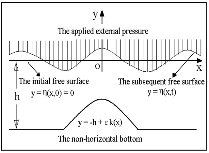
We study the non-linear transient gravity waves inside vast oceans with general topographies. These waves are generated following climate variations simulated by an external pressure acting on the ocean's surface. We use a perturbation method for the study. The present approach necessitates a mild slope of the topography. Quadratic solutions are obtained from nonlinear theory technique and illustrated. The reliability of the nonlinear (quadratic) solution is examined by a comparison between the trace of the bottom and the lowest streamline. The proposed model is shown to be strongly efficient in simulating the considered phenomenon, especially if the slope of the topography is not sharp. The features of the phenomenon under consideration are revealed and discussed mathematically and physically according to the nonlinear theory technique.

References

[1]	B. Le Méhauté, S. Wang, Water waves generated by underwater explosion, Singapore: World Scientific, 1996. https://doi.org/10.1142/2587
[2]	M. S. Abou-Dina, F. M. Hassan, Generation and propagation of nonlinear tsunamis in shallow water by a moving topography, J. Appl. Math. Comput., 177 (2006), 785–806. https://doi.org/10.1016/j.amc.2005.11.033 doi: 10.1016/j.amc.2005.11.033
[3]	I. R. Young, Wind generated ocean waves, Amsterdam: Elsevier, 1999.
[4]	L. H. Holthuijsen, Waves in oceanic and coastal waters, Cambridge: Cambridge University Press, 2007. https://doi.org/10.1017/CBO9780511618536
[5]	S. R. Jayne, L. C. S. Laurent, S. T. Gille, Connections between ocean bottom topography and Earth's climate, Oceanography, 17 (2004), 65–74. https://doi.org/10.5670/oceanog.2004.68 doi: 10.5670/oceanog.2004.68
[6]	L. Chen., J. Y. Yang, L. X. Wu, Topography effects on the seasonal variability of ocean bottom pressure in the North Pacific Ocean, J. Phys. Oceanogr., 53 (2023), 929–94. https://doi.org/10.1175/jpo-d-22-0140.1 doi: 10.1175/jpo-d-22-0140.1
[7]	J. H. Qin, X. H. Cheng, C. C. Yang, N. S. Ou, X. Q. Xiong, Mechanism of interannual variability of ocean bottom pressure in the South Pacific, Clim. Dyn., 59 (2022), 2103–2116. https://doi.org/10.1007/s00382-022-06198-0 doi: 10.1007/s00382-022-06198-0
[8]	J. Y. Yang, K. Chen, The role of wind stress in driving the along‐shelf flow in the northwest Atlantic Ocean, J. Geophys. Res. Oceans, 126 (2021), e2020JC016757. https://doi.org/10.1029/2020JC016757 doi: 10.1029/2020JC016757
[9]	Y. Du, X. L. Dong, X. W. Jiang, Y. H. Zhang, D. Zhu, Q. W. Sun, et al., Ocean surface current multiscale observation mission (OSCOM): Simultaneous measurement of ocean surface current, vector wind, and temperature, Prog. Oceanogr., 193 (2021), 102531. https://doi.org/10.1016/j.pocean.2021.102531 doi: 10.1016/j.pocean.2021.102531
[10]	A. A. Alaidrous, Transmission and reflection of water-wave on a floating ship in vast oceans, Comput. Mater. Con., 67 (2021), 2071–2988. https://doi.org/10.32604/cmc.2021.015159 doi: 10.32604/cmc.2021.015159
[11]	W. Shi, S. H. Zhang, C. Michailides, L. X. Zhang, P. Y. Zhang, X. Li, Experimental investigation of the hydrodynamic effects of breaking waves on monopiles in model scale, J. Mar. Sci. Technol., 28 (2023), 314–325. https://doi.org/10.1007/s00773-023-00926-9 doi: 10.1007/s00773-023-00926-9
[12]	P. Wang, K. Z. Fang, G. Wang, Z. B. Liu, J. W. Sun, Experimental and numerical study of the nonlinear evolution of regular waves over a permeable submerged breakwater, J. Mar. Sci. Eng., 11 (2023), 1610. https://doi.org/10.3390/jmse11081610 doi: 10.3390/jmse11081610
[13]	A. V. Bazilevskii, S. Wongwises, V. A. Kalinichenko, S. Y. Sekerzh-Zen'kovich, Experimental investigation of influence of bottom structure effect on the damping of standing surface waves in a rectangular vessel, Fluid Dynam., 36 (2001), 652–657.
[14]	F. De Serioa, M. Mossa, Experimental study on the hydrodynamics of regular breaking waves, Coast. Eng., 53 (2006), 99–113. https://doi.org/10.1016/j.coastaleng.2005.09.021 doi: 10.1016/j.coastaleng.2005.09.021
[15]	M. S. Abou-Dina, Contribution à l'étude de regime transitoire dans les canaux à houles, PhD Thesis, Université de Grenoble, 1983.
[16]	M. S. Abou-Dina, M. A. Helal, Reduction for the non-linear problem of fluid waves to a system of integro-differential equations with an oceanographic application, J. Comput. Appl. Math., 95 (1998), 65–81. https://core.ac.uk/download/pdf/82146506.pdf
[17]	M. S. Abou-Dina, M. A. Helal, Boundary integral method applied to the transient, nonlinear wave propagation in a fluid with initial free surface elevation, Appl. Math. Model., 24 (2000), 535–549. https://doi.org/10.1016/S0307-904X(99)00054-2 doi: 10.1016/S0307-904X(99)00054-2
[18]	F. M. Hassan, Boundary integral method applied to the propagation of nonlinear gravity waves generated by a moving bottom, Appl. Math. Model., 33 (2009), 451–466. https://doi.org/10.1016/j.apm.2007.11.034 doi: 10.1016/j.apm.2007.11.034
[19]	H. Lamb, Hydrodynamics, 6 Eds., Cambridge: Cambridge University Press, 1932.
[20]	M. S. Abou-Dina, F. M. Hassan, Approximate determination of the transmission and reflection coefficients for water-wave flow over a topography, Appl. Math. Comput., 168 (2005), 283–304. https://doi.org/10.1016/j.amc.2004.08.019 doi: 10.1016/j.amc.2004.08.019
[21]	M. S. Abou-Dina, A. F. Ghaleb, Multiple waves scattering by submerged obstacles in an infinite channel of finite depth. I. streamlines, Eur. J. Mech. B/Fluids, 59 (2016), 37–51. https://doi.org/10.1016/j.euromechflu.2016.04.005 doi: 10.1016/j.euromechflu.2016.04.005
[22]	S. L. Cole, Transient wave produced by flow past a bump, Wave Motion, 7 (1985), 579–587. https://doi.org/10.1016/0165-2125(85)90035-6 doi: 10.1016/0165-2125(85)90035-6
[23]	A. F. Ghaleb, I. A. Z. Hefni, Wave free, two-dimensional, gravity flow of an inviscid fluid over a bump, J. Mech. Theor. Appl., 6 (1987), 463–488.
[24]	S. N. Hanna, M. N. Abdel-Malek, M. B. Abd-el-Malek, Super-critical free surface flow over a trapezoidal obstacle, J. Comput. Appl. Math., 66 (1996), 279–291. https://doi.org/10.1016/0377-0427(95)00160-3 doi: 10.1016/0377-0427(95)00160-3
[25]	T. Nakayama, M. Ikegawa, Finite element analysis of flow over a weir, Comput. Struct., 19 (1984), 129–135. https://doi.org/10.1016/0045-7949(84)90211-6 doi: 10.1016/0045-7949(84)90211-6
[26]	R. W. Yeung, Numerical methods in free-surface flows, Ann. Rev. Fluid Mech., 14 (1982), 395–442. https://doi.org/10.1146/annurev.fl.14.010182.002143 doi: 10.1146/annurev.fl.14.010182.002143
[27]	J. J. Stoker, On radiation conditions, Commun. Pur. Appl. Math., 9 (1956), 577–595. https://doi.org/10.1002/cpa.3160090327 doi: 10.1002/cpa.3160090327
[28]	J. J. Stoker, Water waves: The mathematical theory with application, New York: John Wiley & Sons, Inc., 1957. https://doi.org/10.1002/9781118033159.ch11
[29]	M. S. Abou-Dina, Nonlinear transient gravity waves due to an initial free surface elevation over a topography, J. Comput. Appl. Math., 130 (2001), 173–195. https://doi.org/10.1016/S0377-0427(99)00384-2 doi: 10.1016/S0377-0427(99)00384-2
[30]	M. S. Abou-Dina, M. A. Helal, The influence of a submerged obstacle on an incident wave in stratified shallow water, Eur. J. Mech. B/Fluids, 9 (1990), 545–564.
[31]	M. S. Abou-Dina, M. A. Helal, The effect of a fixed barrier on an incident progressive wave in shallow water, Nuov. Cim. B, 107 (1992), 331–344. https://doi.org/10.1007/BF02728494 doi: 10.1007/BF02728494
[32]	M. S. Abou-Dina, M. A. Helal, The effect of a fixed submerged obstacle on an incident wave in stratified shallow water (mathematical aspects), Nuov. Cim. B, 110 (1995), 927–942. https://doi.org/10.1007/BF02722861 doi: 10.1007/BF02722861
[33]	E. L. Shroye, J. N. Moum, J. D. Nash, Nonlinear internal waves over New Jersey's continental shelf, J. Geophys. Res. Oceans, 116 (2011), e2010JC006332. https://doi.org/10.1029/2010JC006332 doi: 10.1029/2010JC006332
[34]	C. A. Whitwell, N. L. Jones, G. N. Ivey, M. G. Rosevear, M. D. Rayson, Ocean mixing in a shelf sea driven by energetic internal waves, J. Geophys. Res. Oceans, 129 (2024), e2023JC019704. https://doi.org/10.1029/2023JC019704 doi: 10.1029/2023JC019704
[35]	D. P. Marshall, A theoretical model of long Rossby waves in the southern ocean and their interaction with bottom topography, Fluids, 1 (2016), 17. https://doi.org/10.3390/fluids1020017 doi: 10.3390/fluids1020017
[36]	K. Q. Zhang, Analysis of non-linear inundation from sea-level rise using LIDAR data: a case study for south Florida, Climatic Change, 106 (2011), 537–565. https://doi.org/10.1007/s10584-010-9987-2 doi: 10.1007/s10584-010-9987-2
[37]	J. P. Germain, Théorie générale des mouvements d'un fluide parfait pesant en eau peu profonde de profondeur constante, C. R. Acad. Sci. Paris Sér. A-B, 274 (1972), 997–1000.
[38]	Y. L. Chen, J. B. Hung, S. L. Hus, S. C. Hsiao, Y. C.Wu, Interaction of water waves and a submerged parabolic uniform/shear current using RANS model, Math. Probl. Eng., 2014 (2014), 896723. https://doi.org/10.1155/2014/896723 doi: 10.1155/2014/896723
[39]	M. A. Spall, Wind-forced seasonal exchange between marginal seas and the open ocean, J. Phys. Oceanogr., 53 (2023), 763–777. https://doi.org/10.1175/JPO-D-22-0151.1 doi: 10.1175/JPO-D-22-0151.1
[40]	N. Soontiens, C. Subich, M. Stastna, Numerical simulation of super critical trapped internal waves over topography, Phys. Fluids, 22 (2010), 116605. https://doi.org/10.1063/1.3521532 doi: 10.1063/1.3521532
[41]	S. Ahmad, S. F. Aldosary, M. A. Khan, Stochastic solitons of a short-wave intermediate dispersive variable (SIdV) equation, AIMS Mathematics, 9 (2024), 10717–10733. https://doi.org/10.3934/math.2024523 doi: 10.3934/math.2024523
[42]	X. Y. Gao, Two-layer-liquid and lattice considerations through a (3+1)-dimensional generalized Yu-Toda-Sasa-Fukuyama system, Appl. Math. Lett., 152 (2024), 109018. https://doi.org/10.1016/j.aml.2024.109018 doi: 10.1016/j.aml.2024.109018
[43]	X. Y. Gao, Oceanic shallow-water investigations on a generalized Whitham-Broer-Kaup-Boussinesq-Kupershmidt system, Phys. Fluids, 35 (2023), 127106. https://doi.org/10.1063/5.0170506 doi: 10.1063/5.0170506
[44]	X. Y. Gao, Considering the wave processes in oceanography, acoustics and hydrodynamics by means of an extended coupled (2+1)-dimensional Burgers system, Chinese J. Phys., 86 (2023), 572–577. https://doi.org/10.1016/j.cjph.2023.10.051 doi: 10.1016/j.cjph.2023.10.051
[45]	X. Y. Gao, Y. J. Guo, W. R. Shan, Theoretical investigations on a variable-coefficient generalized forced-perturbed Korteweg-de Vries-Burgers model for a dilated artery, blood vessel or circulatory system with experimental support, Commun. Theor. Phys., 75 (2023), 115006. https://doi.org/10.1088/1572-9494%2Facbf24 doi: 10.1088/1572-9494%2Facbf24
[46]	X. H. Wu, Y. T. Gao, Generalized Darboux transformation and solitons for the Ablowitz-Ladik equation in an electrical lattice, Appl. Math. Lett., 137 (2023), 108476. https://doi.org/10.1016/j.aml.2022.108476 doi: 10.1016/j.aml.2022.108476
[47]	Y. Shen, B. Tian, T. Y. Zhou, C. D. Cheng, Multi-pole solitons in an inhomogeneous multi-component nonlinear optical medium, Chaos Soliton. Fract., 171 (2023), 113497. https://doi.org/10.1016/j.chaos.2023.113497 doi: 10.1016/j.chaos.2023.113497
[48]	T. Y. Zhou, B. Tian, Y. Shen, X. T. Gao, Auto-Bä cklund transformations and soliton solutions on the nonzero background for a (3+1)-dimensional Korteweg-de Vries-Calogero-Bogoyavlenskii-Schif equation in a fluid, Nonlinear Dyn., 111 (2023), 8647–8658. http://dx.doi.org/10.1007/s11071-023-08260-w
[49]	X. T. Gao, B. Tian, Water-wave studies on a (2+1)-dimensional generalized variable-coefficient Boiti-Leon-Pempinelli system, Appl. Math. Lett., 128 (2022), 107858.
[50]	X. Bertin, A. de Bakker, A. van Dongeren, G. Coco, G. Andre, F. Ardhuin, et al., Infragravity waves: from diving mechanisms to impacts, Earth-Sci. Rev., 177 (2018), 774–799. https://doi.org/10.1016/j.earscirev.2018.01.002 doi: 10.1016/j.earscirev.2018.01.002
[51]	M. Y. Markina, J. H. P. Studholme. S. K. Gulev, Ocean wind waves climate responses to wintertime north Atlantic atmospheric transient eddies and low-frequency flow, Amer. Meteorolog. Soc., 32 (2019), 5619–5638. https://doi.org/10.1175/JCLI-D-18-0595.1 doi: 10.1175/JCLI-D-18-0595.1
[52]	C. J. Tranter, Integral transforms in mathematical physics, 3 Eds., London: Methuen Co. Ltd., 1966. https://search.worldcat.org/en/title/10766030
[53]	A. H. Nayfeh, Introduction to perturbation techniques, New York: Wiley-Interscience Pub., 1981.
[54]	M. J. Lighthill, An introduction to Fourier analysis and generalized functions, Cambridge: Cambridge University Press, 1958. https://doi.org/10.1017/CBO9781139171427

Reader Comments

Your name:*

Email:*
© 2024 the Author(s), licensee AIMS Press. This is an open access article distributed under the terms of the Creative Commons Attribution License (http://creativecommons.org/licenses/by/4.0)