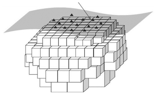
Gravimetry is a discipline of geophysics that deals with observation and interpretation of the earth gravity field. The acquired gravity data serve the study of the earth interior, be it the deep or the near surface one, by means of the inferred subsurface structural density distribution. The subsurface density structure is resolved by solving the gravimetric inverse problem. Diverse methods and approaches exist for solving this non-unique and ill-posed inverse problem. Here, we focused on those methods that do not pre-constrain the number or geometries of the density sources. We reviewed the historical development and the basic principles of the Growth inversion methodology, which belong to the methods based on the growth of the model density structure throughout an iterative exploration process. The process was based on testing and filling the cells of a subsurface domain partition with density contrasts through an iterative mixed weighted adjustment procedure. The procedure iteratively minimized the data misfit residuals jointly with minimizing the total anomalous mass of the model, which facilitated obtaining compact meaningful source bodies of the solution. The applicability of the Growth inversion approach in structural geophysical studies, in geodynamic studies, and in near surface gravimetric studies was reviewed and illustrated. This work also presented the first application of the Growth inversion tool to near surface microgravimetric data with the goal of seeking very shallow cavities in archeological prospection and environmental geophysics.
Citation: Peter Vajda, Jozef Bódi, Antonio G. Camacho, José Fernández, Roman Pašteka, Pavol Zahorec, Juraj Papčo. Gravimetric inversion based on model exploration with growing source bodies (Growth) in diverse earth science disciplines[J]. AIMS Mathematics, 2024, 9(5): 11735-11761. doi: 10.3934/math.2024575
Gravimetry is a discipline of geophysics that deals with observation and interpretation of the earth gravity field. The acquired gravity data serve the study of the earth interior, be it the deep or the near surface one, by means of the inferred subsurface structural density distribution. The subsurface density structure is resolved by solving the gravimetric inverse problem. Diverse methods and approaches exist for solving this non-unique and ill-posed inverse problem. Here, we focused on those methods that do not pre-constrain the number or geometries of the density sources. We reviewed the historical development and the basic principles of the Growth inversion methodology, which belong to the methods based on the growth of the model density structure throughout an iterative exploration process. The process was based on testing and filling the cells of a subsurface domain partition with density contrasts through an iterative mixed weighted adjustment procedure. The procedure iteratively minimized the data misfit residuals jointly with minimizing the total anomalous mass of the model, which facilitated obtaining compact meaningful source bodies of the solution. The applicability of the Growth inversion approach in structural geophysical studies, in geodynamic studies, and in near surface gravimetric studies was reviewed and illustrated. This work also presented the first application of the Growth inversion tool to near surface microgravimetric data with the goal of seeking very shallow cavities in archeological prospection and environmental geophysics.

| [1] | B. Alhijawi, A. Awajan, Genetic algorithms: theory, genetic operators, solutions, and applications, Evol. Intel., 2023. https://doi.org/10.1007/s12065-023-00822-6 |
| [2] | V. Araña, A. G. Camacho, A. Garcia, F. G. Montesinos, I. Blanco, R. Vieira, et al., The internal structure of Tenerife (Canary Islands) based on gravity aeromagnetic and volcanological data, J. Volcanol. Geoth. Res., 103 (2000), 43–64. https://doi.org/10.1016/S0377-0273(00)00215-8 |
| [3] |
V. C. F. Barbosa, J. B. C. Silva, Generalized compact gravity inversion, Geophysics, 59 (1994), 57–68. https://doi.org/10.1190/1.1443534 doi: 10.1190/1.1443534

|
| [4] |
V. C. F. Barbosa, J. B. C. Silva, W. E. Medeiros, Gravity inversion of basements relief using approximate equality constraints on depths, Geophysics, 62 (1997), 1745–1757. https://doi.org/10.1190/1.1444275 doi: 10.1190/1.1444275
|
| [5] |
G. Berrino, A. G. Camacho, 3D gravity inversion by growing bodies and shaping layers at Mt. Vesuvius (Southern Italy), Pure Appl. Geophys., 165 (2008), 1095–1115. https://doi.org/10.1007/s00024-008-0348-2 doi: 10.1007/s00024-008-0348-2
|
| [6] | G. Berrino, P. Vajda, P. Zahorec, A. G. Camacho, V. De Novellis, S. Carlino, et al., Interpretation of spatiotemporal gravity changes accompanying the earthquake of 21 August 2017 on Ischia (Italy), Contrib. Geophys. Geod., 51 (2021), 345–371. https://doi.org/10.31577/congeo.2021.51.4.3 |
| [7] |
H. Bertete-Aguirre, E. Cherkaev, M. Oristaglio, Non-smooth gravity problem with total variation penalization functional, Geophys. J. Int., 149 (2002), 499–507. https://doi.org/10.1046/j.1365-246X.2002.01664.x doi: 10.1046/j.1365-246X.2002.01664.x
|
| [8] | J. Bódi, Inversion of 3D microgravity data for near surface applications for free geometry sources, Rigorous thesis, Comenius University in Bratislava, Slovakia, 2023. |
| [9] |
J. Bódi, P. Vajda, A. G. Camacho, J. Papčo, J. Fernández, On gravimetric detection of thin elongated sources using the growth inversion approach, Surv. Geophys., 44 (2023), 1811–1835. https://doi.org/10.1007/s10712-023-09790-z doi: 10.1007/s10712-023-09790-z
|
| [10] |
O. Boulanger, M. Chouteau, Constraints in 3D gravity inversion, Geophys. Prospect., 49 (2001), 265–280. https://doi.org/10.1046/j.1365-2478.2001.00254.x doi: 10.1046/j.1365-2478.2001.00254.x
|
| [11] | A. G. Camacho, R. Vieira, C. de Toro, Microgravimetric model of the Las Cañadas caldera (Tenerife), J. Volcanol. Geoth. Res., 47 (1991), 75–88. https://doi.org/10.1016/0377-0273(91)90102-6 |
| [12] |
A. G. Camacho, R. Vieira, F. G. Montesinos, V. Cuéllar, A gravimetric 3D Global inversion for cavity detection, Geophys. Prospect., 42 (1994), 113–130. https://doi.org/10.1111/j.1365-2478.1994.tb00201.x doi: 10.1111/j.1365-2478.1994.tb00201.x
|
| [13] |
A. G. Camacho, F. G. Montesinos, R. Vieira, A three-dimensional gravity inversion applied to Sao Miguel Island (Azores), J. Geophys. Res., 102 (1997), 7705–7715. https://doi.org/10.1029/96JB03667 doi: 10.1029/96JB03667
|
| [14] |
A. Camacho, F. Montesinos, R. Vieira, Gravity inversion by means of growing bodies, Geophysics, 65 (2000), 95–101. https://doi.org/10.1190/1.1444729 doi: 10.1190/1.1444729
|
| [15] |
A. Camacho, F. Montesinos, R. Vieira, J. Arnoso, Modelling of crustal anomalies of Lanzarote (Canary Islands) in light of gravity data, Geophys. J. Int., 147 (2001), 403–414. https://doi.org/10.1046/j.0956-540x.2001.01546.x doi: 10.1046/j.0956-540x.2001.01546.x
|
| [16] |
A. G. Camacho, F. G. Montesinos, R. Vieira, A 3-D gravity inversion tool based on exploration of model possibilities, Comput. Geosci., 28 (2002), 191–204. https://doi.org/10.1016/S0098-3004(01)00039-5 doi: 10.1016/S0098-3004(01)00039-5
|
| [17] |
A. G. Camacho, J. C. Nunes, E. Ortíz, Z. Franca, R. Vieira, Gravimetric determination of an intrusive complex under the island of Faial (Azores): some methodological improvements, Geophys. J. Int., 171 (2007), 478–494. https://doi.org/10.1111/j.1365-246X.2007.03539.x doi: 10.1111/j.1365-246X.2007.03539.x
|
| [18] | A. G. Camacho, J. Fernández, P. J. González, J. B. Rundle, J. F. Prieto, A. Arjona, Structural results for La Palma island using 3-D gravity inversion, J. Geophys. Res., 114 (2009), B05411. https://doi.org/10.1029/2008JB005628 |
| [19] | A. Camacho, J. Fernández, J. Gottsmann, The 3-D gravity inversion package GROWTH 2.0 and its application to Tenerife Island, Spain, Comput. Geosci., 37 (2011), 621–633. https://doi.org/10.1016/j.cageo.2010.12.003 |
| [20] | A. G. Camacho, J. Fernández, J. Gottsmann, A new gravity inversion method for multiple subhorizontal discontinuity interfaces and shallow basins, J. Geophys. Res., 116 (2011), B02413. https://doi.org/10.1029/2010JB008023 |
| [21] | A. G. Camacho, P. J. González, J. Fernández, G. Berrino, Simultaneous inversion of surface deformation and gravity changes by means of extended bodies with a free geometry: application to deforming calderas, J. Geophys. Res., 116 (2011), B10. https://doi.org/10.1029/2010JB008165 |
| [22] | A. G. Camacho, E. Carmona, A. García-Jerez, F. Sánchez-Martos, J. F. Prieto, J. Fernández, et al., Structure of alluvial valleys from 3-D gravity inversion: the Low Andarax Valley (Almería, Spain) test case, Pure Appl. Geophys., 172 (2015), 3107–3121. https://doi.org/10.1007/s00024-014-0914-8 |
| [23] |
A. G. Camacho, J. Fernández, Modeling 3D free-geometry volumetric sources associated to geological and anthropogenic hazards from space and terrestrial geodetic data, Remote Sens., 11 (2019), 2042. https://doi.org/10.3390/rs11172042 doi: 10.3390/rs11172042
|
| [24] | A. G. Camacho, J. F. Prieto, E. Ancochea, J. Fernández, Deep volcanic morphology below Lanzarote, Canaries, from gravity inversion: new results for Timanfaya and implications, J. Volcanol. Geoth. Res., 369 (2019), 64–79. https://doi.org/10.1016/j.jvolgeores.2018.11.013 |
| [25] |
A. G. Camacho, J. Fernández, S. V. Samsonov, K. F. Tiampo, M. Palano, 3D multi-source model of elastic volcanic ground deformation, Earth Planet. Sci. Lett., 547 (2020), 116445. https://doi.org/10.1016/j.epsl.2020.116445 doi: 10.1016/j.epsl.2020.116445
|
| [26] |
A. G. Camacho, J. F. A. Aparicio, E. Ancochea, J. Fernández, Upgraded GROWTH 3.0 software for structural gravity inversion and application to El Hierro (Canary Islands), Comput. Geosci., 150 (2021), 104720. https://doi.org/10.1016/j.cageo.2021.104720 doi: 10.1016/j.cageo.2021.104720
|
| [27] |
A. G. Camacho, P. Vajda, C. A. Miller, J. Fernández, A free-geometry geodynamic modelling of surface gravity changes using Growth-dg software, Sci. Rep., 11 (2021), 23442. https://doi.org/10.1038/s41598-021-02769-z doi: 10.1038/s41598-021-02769-z
|
| [28] |
A. G. Camacho, P. Vajda, J. Fernández, GROWTH-23: an integrated code for inversion of complete Bouguer gravity anomaly or temporal gravity changes, Comput. Geosci., 182 (2024), 105495. https://doi.org/10.1016/j.cageo.2023.105495 doi: 10.1016/j.cageo.2023.105495
|
| [29] |
F. Cannavò, A. G. Camacho, P. J. González, M. Mattia, G. Puglisi, J. Fernández, Real time tracking of magmatic intrusions by means of ground deformation modeling during volcanic crises, Sci. Rep., 5 (2015), 10970. https://doi.org/10.1038/srep10970 doi: 10.1038/srep10970
|
| [30] |
Z. Chen, X. Meng, L. Guo, G. Liu, GICUDA: a parallel program for 3D correlation imaging of large scale gravity and gravity gradiometry data on graphics processing units with CUDA, Comput. Geosci., 46 (2012), 119–128. https://doi.org/10.1016/j.cageo.2012.04.017 doi: 10.1016/j.cageo.2012.04.017
|
| [31] |
Z. Chen, X. Meng, S. Zhang, 3D gravity interface inversion constrained by a few points and its GPU acceleration, Comput. Geosci., 84 (2015), 20–28. https://doi.org/10.1016/j.cageo.2015.08.002 doi: 10.1016/j.cageo.2015.08.002
|
| [32] | C. G. Farquharson, M. R. Ash, H. G Miller, Geologically constrained gravity inversion for the Voisey's Bay Ovoid deposit, Lead. Edge, 27 (2008), 64–69. https://doi.org/10.1190/1.2831681 |
| [33] | J. Fernández, J. F. Prieto, J. Escayo, A. G. Camacho, F. Luzón, K. F. Tiampo, et al., Modeling the two-and three-dimensional displacement field in Lorca, Spain, subsidence and the global implications, Sci. Rep., 8 (2018), 14782. https://doi.org/10.1038/s41598-018-33128-0 |
| [34] | J. Fernández, J. Escayo, Z. Hu, A. G. Camacho, S. V. Samsonov, J. F. Prieto, et al., Detection of volcanic unrest onset in La Palma, Canary Islands, evolution and implications, Sci. Rep., 11 (2021), 2540. https://doi.org/10.1038/s41598-021-82292-3 |
| [35] | J. Fernández, J. Escayo, A. G. Camacho, M. Palano, J. F. Prieto, Z. Hu, et al., Shallow magmatic intrusion evolution below La Palma before and during the 2021 eruption, Sci. Rep., 12 (2022), 20257. https://doi.org/10.1038/s41598-022-23998-w |
| [36] | J. Fullea, J. C. Afonso, J. A. D. Connolly, M. Fernàndez, D. Garcia-Castellanos, H. Zeyen, LitMod3D: an interactive 3D software to model the thermal, compositional, density, rheological, and seismological structure of the lithosphere and sublithospheric upper mantle, Geochem. Geophys. Geosy., 10 (2009), Q08019. https://doi.org/10.1029/2009GC002391 |
| [37] |
M. H. Ghalehnoee, A. Ansari, A. Ghorbani, Improving compact gravity inversion using new weighting functions, Geophys. J. Int., 208 (2017), 546–560. https://doi.org/10.1093/gji/ggw413 doi: 10.1093/gji/ggw413
|
| [38] |
D. Gómez-Ortiz, B. N. P. Agarwal, 3DINVER.M: a MATLAB program to invert the gravity anomaly over a 3D horizontal density interface by Parker–Oldenburg's algorithm, Comput. Geosci., 31 (2005), 513–520. https://doi.org/10.1016/j.cageo.2004.11.004 doi: 10.1016/j.cageo.2004.11.004
|
| [39] | J. Gottsmann, L. Wooller, J. Martí, J. Fernández, A. G. Camacho, P. J. Gonzalez, et al., New evidence for the reawakening of Teide volcano, Geophys. Res. Lett., 33 (2006), L20311. https://doi.org/10.1029/2006GL027523 |
| [40] | J. Gottsmann, A. G. Camacho, J. Martí, L. Wooller, J. Fernández, A. García, et al., Shallow structure beneath the Central Volcanic Complex of Tenerife from new gravity data: implications for its evolution and recent reactivation, Phys. Earth Planet. Int., 168 (2008), 212–230. https://doi.org/10.1016/j.pepi.2008.06.020 |
| [41] |
A. Guillen, V. Menichetti, Gravity and magnetic inversion with minimization of a specific functional, Geophysics, 49 (1984), 1354–1360. https://doi.org/10.1190/1.1441761 doi: 10.1190/1.1441761
|
| [42] |
J. R. Kennedy, J. D. Larsen, Heavy: software for forward modeling gravity change from MODFLOW output, Environ. Modell. Softw., 165 (2023), 105714. https://doi.org/10.1016/j.envsoft.2023.105714 doi: 10.1016/j.envsoft.2023.105714
|
| [43] |
C. Klesper, IVIS-3D: a tool for interactive 3D-visualisation of gravity models, Phys. Chem. Earth, 23 (1998), 279–283. https://doi.org/10.1016/S0079-1946(98)00025-1 doi: 10.1016/S0079-1946(98)00025-1
|
| [44] |
R. A. Krahenbuhl, Y. Li, Inversion of gravity data using a binary formulation, Geophys. J. Int., 167 (2006), 543–556. https://doi.org/10.1111/j.1365-246X.2006.03179.x doi: 10.1111/j.1365-246X.2006.03179.x
|
| [45] | B. J. Last, K. Kubik, Compact gravity inversion, Geophysics, 48 (1983), 713–721. https://doi.org/10.1190/1.1441501 |
| [46] |
P. G. Lelievre, D. W. Oldenburg, A comprehensive study of including structural information in geophysical inversions, Geophys. J. Int., 178 (2009), 623–637. https://doi.org/10.1111/j.1365-246X.2009.04188.x doi: 10.1111/j.1365-246X.2009.04188.x
|
| [47] |
P. G. Lelièvre, R. Bijani, C. G. Farquharson, Joint inversion using multi-objective global optimization methods, 78th EAGE Conference and Exhibition, 2016 (2016), 1–5. https://doi.org/10.3997/2214-4609.201601655 doi: 10.3997/2214-4609.201601655
|
| [48] |
Y. Li, D. W. Oldenburg, 3-D inversion of gravity data, Geophysics, 63 (1998), 109–119. https://doi.org/10.1190/1.1444302 doi: 10.1190/1.1444302
|
| [49] | S. Mallick, Optimization using genetic algorithms–Methodology with examples from seismic waveform inversion (chapter), In: Y. H. Chemin, Genetic algorithms: theory, design and programming, IntechOpen, 2024. https://doi.org/10.5772/intechopen.113897 |
| [50] | C. M. Martins, W. A. Lima, V. C. F. Barbosa, J. B. C. Silva, Total variation regularization for depth-to-basement estimate: Part 1–Mathematical details and applications, Geophysics, 76 (2011), I1–I12. https://doi.org/10.1190/1.3524286 |
| [51] | C. A. Miller, G. Williams-Jones, D. Fournier, J. Witter, 3D gravity inversion and thermodynamic modelling reveal properties of shallow silicic magma reservoir beneath Laguna del Maule, Chile, Earth Planet. Sci. Lett., 459 (2017), 14–27. https://doi.org/10.1016/j.epsl.2016.11.007 |
| [52] |
C. A. Miller, H. Le Mével, G. Currenti, G. Williams-Jones, B. Tikoff, Microgravity changes at the Laguna del Maule volcanic field: Magma-induced stress changes facilitate mass addition, J. Geophys. Res. Solid Earth, 122 (2017), 3179–3196. https://doi.org/10.1002/2017JB014048 doi: 10.1002/2017JB014048
|
| [53] |
O. F. Mojica, A. Bassrei, Regularization parameter selection in the 3D gravity inversion of the basement relief using GCV: a parallel approach, Comput. Geosci., 82 (2015), 205–213. https://doi.org/10.1016/j.cageo.2015.06.013 doi: 10.1016/j.cageo.2015.06.013
|
| [54] | F. G. Montesinos, A. G. Camacho, R. Vieira, Analysis of gravimetric anomalies in Furnas caldera (Saô Miguel, Azores), J. Volcanol. Geoth. Res., 92 (1999), 67–81. https://doi.org/10.1016/S0377-0273(99)00068-2 |
| [55] |
F. G. Montesinos, A. G. Camacho, J. C. Nunes, C. S. Oliveira, R. Vieira, A 3-D gravity model for a volcanic crater in Terceira Island (Azores), Geophys. J. Int., 154 (2003), 393–406. https://doi.org/10.1046/j.1365-246X.2003.01960.x doi: 10.1046/j.1365-246X.2003.01960.x
|
| [56] | F. G. Montesinos, J. Arnoso, R. Vieira, Using a genetic algorithm for 3-D inversion of gravity data in Fuerteventura (Canary Islands), Int. J. Earth Sci. (Geol. Rundsch.), 94 (2005), 301–316. https://doi.org/10.1007/s00531-005-0471-6 |
| [57] | J. C. Nunes, A. Camacho, Z. França, F. G. Montesinos, M. Alves, R. Vieira, et al., Gravity anomalies and crustal signature of volcano-tectonic structures of Pico Island (Azores), J. Volcanol. Geoth. Res., 156 (2006), 55–70. https://doi.org/10.1016/j.jvolgeores.2006.03.023 |
| [58] |
E. Oksum, Grav3CH_inv: A GUI-based MATLAB code for estimating the 3-D basement depth structure of sedimentary basins with vertical and horizontal density variation, Comput. Geosci., 155 (2021), 104856. https://doi.org/10.1016/j.cageo.2021.104856 doi: 10.1016/j.cageo.2021.104856
|
| [59] |
V. C. Oliveira, V. C. F. Barbosa, 3-D radial gravity gradient inversion, Geophys. J. Int., 195 (2013), 883–902. https://doi.org/10.1093/gji/ggt307 doi: 10.1093/gji/ggt307
|
| [60] |
L. B. Pedersen, Constrained inversion of potential field data, Geophys. Prosp., 27 (1979), 726–748. https://doi.org/10.1111/j.1365-2478.1979.tb00993.x doi: 10.1111/j.1365-2478.1979.tb00993.x
|
| [61] |
D. Phillips, A technique for the numerical solution of certain integral equations of the first kind, J. ACM, 9 (1962), 84–97. https://doi.org/10.1145/321105.321114 doi: 10.1145/321105.321114
|
| [62] | R. Pašteka, M. Terray, M. Hajach, M. Pašiaková, Výsledky geofyzikálneho (mikro-gravimetrického) prieskumu interiéru kostola Sv. Mikuláša v Trnave, unpublished work, 2006. |
| [63] | R. Pašteka, J. Mikuška, M. Hajach, M. Pašiaková, Microgravity measurements and GPR technique in the search for medieval crypts: a case study from the St. Nicholas church in Trnava, SW Slovakia, Proceedings of the Archaeological Prospection 7th Conference in Nitra, 41 (2007), 222–224. |
| [64] |
R. Pašteka, F. P. Richter, R. Karcol, K. Brazda, M. Hajach, Regularized derivatives of potential fields and their role in semiautomated interpretation methods, Geophys. Prospect., 57 (2009), 507–516. https://doi.org/10.1111/j.1365-2478.2008.00780.x doi: 10.1111/j.1365-2478.2008.00780.x
|
| [65] | R. Pašteka, J. Pánisová, P. Zahorec, J. Papčo, J. Mrlina, M. Fraštia, et al., Microgravity method in archaeological prospection: methodical comments on selected case studies from crypt and tomb detection, Archaeol. Prospect., 27 (2020), 415–431. https://doi.org/10.1002/arp.1787 |
| [66] | M. Pick, J. Picha, V. Vyskočil, Theory of the earth's gravity field, Elsevier, 1973. |
| [67] |
I. Prutkin, P. Vajda, M. Bielik, V. Bezák, R. Tenzer, Joint interpretation of gravity and magnetic data in the Kolárovo anomaly region by separation of sources and the inversion method of local corrections, Geol. Carpath., 65 (2014), 163–174. https://doi.org/10.2478/geoca-2014-0011 doi: 10.2478/geoca-2014-0011
|
| [68] |
I. Prutkin, P. Vajda, J. Gottsmann, The gravimetric picture of magmatic and hydrothermal sources driving hybrid unrest on Tenerife in 2004/5, J. Volcanol. Geoth. Res., 282 (2014), 9–18. https://doi.org/10.1016/j.jvolgeores.2014.06.003 doi: 10.1016/j.jvolgeores.2014.06.003
|
| [69] | I. Prutkin, P. Vajda, T. Jahr, F. Bleibinhaus, P. Novák, R. Tenzer, Interpretation of gravity and magnetic data with geological constraints for 3D structure of the Thuringian Basin, Germany, J. Appl. Geophys., 136 (2017), 35–41. https://doi.org/10.1016/j.jappgeo.2016.10.039 |
| [70] |
A. B. Reid, J. M. Allsop, H. Granser, A. J. Millet, I. W. Somerton, Magnetic interpretation in three dimensions using Euler deconvolution, Geophysics, 55 (1990), 80–91. https://doi.org/10.1190/1.1442774 doi: 10.1190/1.1442774
|
| [71] | R. M. René, Gravity inversion using open, reject, and "shape‐of‐anomaly" fill criteria, Geophysics, 51 (1986), 889–1033. https://doi.org/10.1190/1.1442157 |
| [72] | D. F. Santos, J. B. C. Silva, C. M. Martins, R. C. S. Santos, L. C. Ramos, A. C. M. Araújo, Efficient gravity inversion of discontinuous basement relief, Geophysics, 80 (2015), G95–G106. https://doi.org/10.1190/geo2014-0513.1 |
| [73] | S. V. Samsonov, K. F. Tiampo, A. G. Camacho, J. Fernández, P. J. González, Spatiotemporal analysis and interpretation of 1993–2013 ground deformation at Campi Flegrei, Italy, observed by advanced DInSAR, Geophys. Res. Lett., 41 (2014), 6101–6108. https://doi.org/10.1002/2014GL060595 |
| [74] |
P. Shamsipour, D. Marcotte, M. Chouteau, 3D stochastic joint inversion of gravity and magnetic data, J. Appl. Geophys., 79 (2012), 27–37. https://doi.org/10.1016/j.jappgeo.2011.12.012 doi: 10.1016/j.jappgeo.2011.12.012
|
| [75] |
K. Snopek, U. Casten, 3GRAINS: 3D Gravity Interpretation Software and its application to density modeling of the Hellenic subduction zone, Comput. Geosci., 32 (2006), 592–603. https://doi.org/10.1016/j.cageo.2005.08.008 doi: 10.1016/j.cageo.2005.08.008
|
| [76] | M. Terray, Správa z georadarového prieskumu Dómu sv. Mikuláša v Trnave, unpublished work, 2006. |
| [77] | C. Tiede, A. G. Camacho, C. Gerstenecker, J. Fernández, I. Suyanto, Modelling the crust at Merapi volcano area, Indonesia, via the inverse gravimetric problem, Geochem. Geophy. Geosy., 6 (2005), Q09011. https://doi.org/10.1029/2005GC000986 |
| [78] | C. Tiede, J. Fernández, C. Gerstenecker, K. F. Tiampo, A hybrid model for the summit region of merapi volcano, Java, Indonesia, derived from gravity changes and deformation measured between 2000 and 2002, In: D. Wolf, J. Fernández, Deformation and gravity change: indicators of isostasy, tectonics, volcanism, and climate change, Pageoph Topical Volumes, Birkhäuser, (2007), 837–850. https://doi.org/10.1007/978-3-7643-8417-3_12 |
| [79] | A. N. Tikhonov, V. A. Arsenin, Solutions of ill-posed problems, Winston and Sons, Washington, 1977. https://doi.org/10.2307/2006360 |
| [80] | L. Uieda, V. C. F. Barbosa, Robust 3D gravity gradient inversion by planting anomalous densities, Geophysics, 77 (2012), G55–G66. https://doi.org/10.1190/GEO2011-0388.1 |
| [81] |
P. Vajda, P. Vaníček, B. Meurers, A new physical foundation for anomalous gravity, Stud. Geophys. Geod., 50 (2006), 189–216. https://doi.org/10.1007/s11200-006-0012-1 doi: 10.1007/s11200-006-0012-1
|
| [82] | P. Vajda, I. Foroughi, P. Vaníček, R. Kingdon, M. Santos, M. Sheng, et al., Topographic gravimetric effects in earth sciences: Review of origin, significance and implications, Earth-Sci. Rev., 211 (2020), 103428. https://doi.org/10.1016/j.earscirev.2020.103428 |
| [83] |
P. Vajda, P. Zahorec, C. A. Miller, H. Le Mével, J. Papčo, A. G. Camacho, Novel treatment of the deformation–induced topographic effect for interpretation of spatiotemporal gravity changes: Laguna del Maule (Chile), J. Volcanol. Geoth. Res., 414 (2021), 107230. https://doi.org/10.1016/j.jvolgeores.2021.107230 doi: 10.1016/j.jvolgeores.2021.107230
|
| [84] |
P. Vajda, A. G. Camacho, J. Fernández, Benefits and limitations of the growth inversion approach in volcano gravimetry demonstrated on the revisited Tenerife 2004/5 unrest, Surveys Geophys., 44 (2023), 527–554. https://doi.org/10.1007/s10712-022-09738-9 doi: 10.1007/s10712-022-09738-9
|
| [85] |
S. Vatankhah, V. E. Ardestani, S. S. Niri, R. S. Renaut, H. Kabirzadeh, IGUG: a MATLAB package for 3D inversion of gravity data using graph theory, Comput. Geosci., 128 (2019), 19–29. https://doi.org/10.1016/j.cageo.2019.03.008 doi: 10.1016/j.cageo.2019.03.008
|
| [86] |
E. J. Wahyudi, D. Santoso, W. G. A. Kadir, S. Alawiyah, Designing a genetic algorithm for efficient calculation in time-lapse gravity inversion, J. Eng. Tech. Sci., 46 (2014), 58–77. https://doi.org/10.5614/j.eng.technol.sci.2014.46.1.4 doi: 10.5614/j.eng.technol.sci.2014.46.1.4
|
| [87] | R. A. Wildman, G. A. Gazonas, Gravitational and magnetic anomaly inversion using a tree-based geometry representation, Geophysics, 74 (2009), I23–I35. https://doi.org/10.1190/1.3110042 |
| [88] |
Y. Tian, X. Ke, Y. Wang, DenInv3D: a geophysical software for three-dimensional density inversion of gravity field data, J. Geophys. Eng., 15 (2018), 354–365. https://doi.org/10.1088/1742-2140/aa8caf doi: 10.1088/1742-2140/aa8caf
|
| [89] | P. Zahorec, R. Pašteka, J. Papčo, R. Putiška, A. Mojzeš, D. Kušnirák, et al., Mapping hazardous cavities over collapsed coal mines: case study experiences using the microgravity method, Near Surface Geophys., 19 (2021), 353–364. https://doi.org/10.1002/nsg.12139 |
| [90] | D. Zidarov, Inverse gravimetric problem in geoprospecting and geodesy, Elsevier Science Publ. Co., 1990. |


Figures(7)

Peter Vajda, Jozef Bódi, Antonio G. Camacho, José Fernández, Roman Pašteka, Pavol Zahorec, Juraj Papčo. Gravimetric inversion based on model exploration with growing source bodies (Growth) in diverse earth science disciplines[J]. AIMS Mathematics, 2024, 9(5): 11735-11761. doi: 10.3934/math.2024575


 DownLoad: