Shock stability of a novel flux splitting scheme

Weiping Wei; Youlin Shang; Hongwei Jiao; Pujun Jia; Weiping Wei; Youlin Shang; Hongwei Jiao; Pujun Jia

doi:10.3934/math.2024364

AIMS Mathematics

2024, Volume 9, Issue 3: 7511-7528. doi: 10.3934/math.2024364

Previous Article Next Article

Research article

Shock stability of a novel flux splitting scheme

1.
College of Information Engineering, Henan University of Science and Technology, Luoyang 471023, China
2.
School of Mathematical Sciences, Henan Institute of Science and Technology, Xinxiang 453003, China
3.
School of Mathematics and Statistics, Henan University of Science and Technology, Luoyang 471023, China

Received: 19 October 2023 Revised: 24 January 2024 Accepted: 05 February 2024 Published: 21 February 2024
MSC : 58J45, 76J20

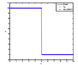
This article introduced the HLL-CPS-T flux splitting scheme, which is characterized by low dissipation and robustness. A detailed theoretical analysis of the dissipation and shock stability of this scheme was provided. In comparison to Toro's TV flux splitting scheme, the HLL-CPS-T scheme not only exhibits accurate capture of contact discontinuity, but also demonstrates superior shock stability, as evidenced by its absence of 'carbuncle' phenomenon. Through an examination of the disturbance attenuation properties of physical quantities in the TV and HLL-CPS-T schemes, an inference was derived: The shock stability condition for an upwind method in the velocity perturbation was damped. Theoretical analysis was given to verify the reasonableness of this inference. Numerical experiments were carefully selected to test the robustness of the new splitting scheme.
- low dissipation,
- flux splitting scheme,
- shock stability,
- upwind method
Citation: Weiping Wei, Youlin Shang, Hongwei Jiao, Pujun Jia. Shock stability of a novel flux splitting scheme[J]. AIMS Mathematics, 2024, 9(3): 7511-7528. doi: 10.3934/math.2024364

Related Papers:

Abstract

This article introduced the HLL-CPS-T flux splitting scheme, which is characterized by low dissipation and robustness. A detailed theoretical analysis of the dissipation and shock stability of this scheme was provided. In comparison to Toro's TV flux splitting scheme, the HLL-CPS-T scheme not only exhibits accurate capture of contact discontinuity, but also demonstrates superior shock stability, as evidenced by its absence of 'carbuncle' phenomenon. Through an examination of the disturbance attenuation properties of physical quantities in the TV and HLL-CPS-T schemes, an inference was derived: The shock stability condition for an upwind method in the velocity perturbation was damped. Theoretical analysis was given to verify the reasonableness of this inference. Numerical experiments were carefully selected to test the robustness of the new splitting scheme.

References

[1]	G. Tchuen, M. Fogue, Y. Burtschell, D. Zeitoun, G. Ben-Dor, Shock-on-shock interactions over double-wedges: Comparison between inviscid, viscous and nonequilibrium hypersonic flow, Berlin: Springer, 2009. https://doi.org/10.1007/978-3-540-85181-3_114
[2]	N. H. Johannesen, Experiments on two-dimensional supersonic flow in corners and over concave surfaces, Lond. Edinb. Dubl. Phil. Mag. J. Sci., 43 (1952), 568–580. https://doi.org/10.1080/14786440508520212 doi: 10.1080/14786440508520212
[3]	G. C. Zha, E. Bilgen, Numerical solutions of Euler equations by using a new flux vector splitting scheme, Int. J. Numer. Methods Fluids, 17 (1993), 115–144. https://doi.org/10.1002/fld.1650170203 doi: 10.1002/fld.1650170203
[4]	D. J. Singh, A. Kumar, S. N. Tiwari, Numerical simulation of shock impingement on blunt cowl lip in viscous hypersonic, Numer. Heat Tr. A Appl., 20 (1991), 329–344. https://doi.org/10.1080/10407789108944825 doi: 10.1080/10407789108944825
[5]	J. W. Shen, Shock wave solutions of the compound Burgers-Korteweg-de Vries equation, Appl. Math. Comput., 196 (2008), 842–849. https://doi.org/10.1016/j.amc.2007.07.029 doi: 10.1016/j.amc.2007.07.029
[6]	B. Barker, H. Freistühler, K. Zumbrun, Convex entropy, Hopf bifurcation, and viscous and inviscid shock stability, Arch Ration. Mech. Anal., 217 (2015), 309–372. https://doi.org/10.1007/s00205-014-0838-6 doi: 10.1007/s00205-014-0838-6
[7]	B. Xue, F. Li, X. G. Geng, Quasi-periodic solutions of coupled KDV type equations, J. Nonlinear Math. Phys., 20 (2013), 61–77. http://dx.doi.org/10.1080/14029251.2013.792472 doi: 10.1080/14029251.2013.792472
[8]	B. Xue, X. G. Geng, F. Li, Quasiperiodic solutions of Jaulent-Miodek equations with a negative flow, J. Math. Phys., 53 (2012), 063710. https://doi.org/10.1063/1.4729868 doi: 10.1063/1.4729868
[9]	R. T. Alqahtani, J. C. Ntonga, E. Ngondiep, Stability analysis and convergence rate of a two-step predictor-corrector approach for shallow water equations with source terms, AIMS Mathematics, 8 (2023), 9265–9289. https://doi.org/10.3934/math.2023465 doi: 10.3934/math.2023465
[10]	C. Caginalp, Minimization solutions to conservation laws with non-smooth and non-strictly convex flux, AIMS Mathematics, 3 (2018), 96–130. https://doi.org/10.3934/Math.2018.1.96 doi: 10.3934/Math.2018.1.96
[11]	E. F. Toro, C. E. Castro, D. Vanzo, A. Siviglia, A flux-vector splitting scheme for the shallow water equations extended to high-order on unstructured meshes, Int. J. Numer. Methods Fluids, 94 (2022), 1679–1705. https://doi.org/10.1002/fld.5099 doi: 10.1002/fld.5099
[12]	B. Parent, Positivity-preserving flux difference splitting schemes, J. Comput. Phys., 243 (2013), 194–209. https://doi.org/10.1016/j.jcp.2013.02.048 doi: 10.1016/j.jcp.2013.02.048
[13]	W. T. Roberts, The behavior of difference splitting schemes near slowly moving shock waves, J. Comput. Phys., 90 (1990), 141–160. https://doi.org/10.1016/0021-9991(90)90200-K doi: 10.1016/0021-9991(90)90200-K
[14]	E. F. Toro, Riemann solvers and numerical methods for fluid dynamic, Berlin: Springer, 1997. https://doi.org/10.1007/978-3-540-49834-6
[15]	G. Tchuen, Y. Burtschell, D. E. Zeitoun, Computation of non-equilibrium hypersonic flow with artificially upstream flux vector splitting (AUFS) scheme, Int. J. Comput. Fluid Dyn., 22 (2008), 209–220. https://doi.org/10.1080/10618560701766525 doi: 10.1080/10618560701766525
[16]	J. L. Steger, R. F. Warming, Flux vector splitting of the inviscid gas dynamic equations with application to finite difference methods, J. Comput. Phys., 40 (1981), 263–293. https://doi.org/10.1016/0021-9991(81)90210-2 doi: 10.1016/0021-9991(81)90210-2
[17]	E. F. Toro, M. E. Vázquez-Cendón, Flux splitting schemes for the Euler equations, Comput. Fluids, 70 (2012), 1–12. https://doi.org/10.1016/j.compfluid.2012.08.023 doi: 10.1016/j.compfluid.2012.08.023
[18]	J. C. Mandal, V. Panwar, Robust HLL-type Riemann solver capable of resolving contact discontinuity, Comput. Fluids, 63 (2012), 148–164. https://doi.org/10.1016/j.compfluid.2012.04.005 doi: 10.1016/j.compfluid.2012.04.005
[19]	W. J. Xie, H. Li, Z. Y. Tian, S. Pan, A low diffusion flux splitting method for inviscid compressible flows, Comput. Fluids, 112 (2015), 83–93. https://doi.org/10.1016/j.compfluid.2015.02.004 doi: 10.1016/j.compfluid.2015.02.004
[20]	K. Chakravarthy, D. Chakraborty, Modified SLAU2 scheme with enhanced shock stability, Comput. Fluids, 100 (2014), 176–184. https://doi.org/10.1016/j.compfluid.2014.04.015 doi: 10.1016/j.compfluid.2014.04.015
[21]	H. Kim, M. S. Liou, Adaptive Cartesian cut-cell sharp interface method (aC3SIM) for three-dimensional multi-phase flows, Shock Waves, 29 (2019), 1023–1041. https://doi.org/10.1007/s00193-019-00902-6 doi: 10.1007/s00193-019-00902-6
[22]	A. V. Fedorov, A. A. Ryzhov, V. G. Soudakov, S. V. Utyuzhnikov, Numerical simulation of the effect of local volume energy supply on high-speed boundary layer stability, Comput. Fluids, 100 (2014), 130–137. https://doi.org/10.1016/j.compfluid.2014.04.026 doi: 10.1016/j.compfluid.2014.04.026
[23]	M. Pandolfi, D. D'Ambrosio, Numerical instabilities in upwind methods: Analysis and cures for the 'carbuncle' phenomenon, J. Comput. Phys., 166 (2001), 271–301. https://doi.org/10.1006/jcph.2000.6652 doi: 10.1006/jcph.2000.6652
[24]	M. S. Liou, C. J. Steffen, A new flux spitting scheme, J. Comput. Phys., 107 (1993), 23–39. https://doi.org/10.1006/jcph.1993.1122 doi: 10.1006/jcph.1993.1122
[25]	M. S. Liou, Mass flux schemes and connection to shock instability, J. Comput. Phys., 160 (2000), 623–648. https://doi.org/10.1006/jcph.2000.6478 doi: 10.1006/jcph.2000.6478
[26]	D. Sun, C. Yan, F. Qu, R. Du, A robust flux splitting method with low dissipation for all-speed flows, Int. J. Numer. Methods Fluids, 84 (2016), 3–18. https://doi.org/10.1002/fld.4337 doi: 10.1002/fld.4337
[27]	N. Fleischmann, S. Adami, X. Y. Hu, N. A. Adams, A low dissipation method to cure the grid-aligned shock instability, J. Comput. Phys., 401 (2020) 109004. https://doi.org/10.1016/j.jcp.2019.109004 doi: 10.1016/j.jcp.2019.109004
[28]	N. Fleischmann, S. Adami, N. A. Adams, A shock-stable modification of the HLLC Riemann solver with reduced numerical dissipation. J. Comput. Phys., 423 (2020) 109762. https://doi.org/10.1016/j.jcp.2020.109762 doi: 10.1016/j.jcp.2020.109762
[29]	F. Kemm, Numerical investigation of Mach number consistent Roe solvers for the Euler equations of gas dynamics, J. Comput. Phys., 477 (2023), 111947. https://doi.org/10.1016/j.jcp.2023.111947 doi: 10.1016/j.jcp.2023.111947
[30]	M. S. Liou, A sequel to AUSM, Part Ⅱ: AUSM+-up for all speeds, J. Comput. Phys., 214 (2006), 137–170. https://doi.org/10.1016/j.jcp.2005.09.020 doi: 10.1016/j.jcp.2005.09.020
[31]	K. Xu, Z.W. Li, Dissipative mechanism in Godunov-type schemes, Int. J. Numer. Methods Fluids, 37 (2001), 1–22. https://doi.org/10.1002/fld.160 doi: 10.1002/fld.160
[32]	M. Sun, K.Takayama, An artificially upstream flux vector splitting scheme for the Euler equations, J. Comput. Phys., 189 (2003), 305–329. https://doi.org/10.1016/S0021-9991(03)00212-2 doi: 10.1016/S0021-9991(03)00212-2
[33]	J. J. Quirk, A contribution to the great Riemann solver debate, Int. J. Numer. Methods Fluids, 18 (1994), 555–574. https://doi.org/ 10.1002/fld.1650180603 doi: 10.1002/fld.1650180603
[34]	P. D. Lax, Hyperbolic systems of conservation laws and the mathematical theory of shock waves, Philadelphia: SIAM, 1973. https://doi.org/10.1137/1.9781611970562

Reader Comments

Your name:*

Email:*
© 2024 the Author(s), licensee AIMS Press. This is an open access article distributed under the terms of the Creative Commons Attribution License (http://creativecommons.org/licenses/by/4.0)